Learning Objectives

• Understand gradient descent intuition
• Choose appropriate learning rates
• Compare batch GD vs SGD
• Implement gradient descent from scratch

Theory

The Core Idea: Finding the Bottom of a Valley

Gradient descent is the workhorse algorithm behind training most machine learning models. The goal is simple: find the parameters that minimize a loss function.

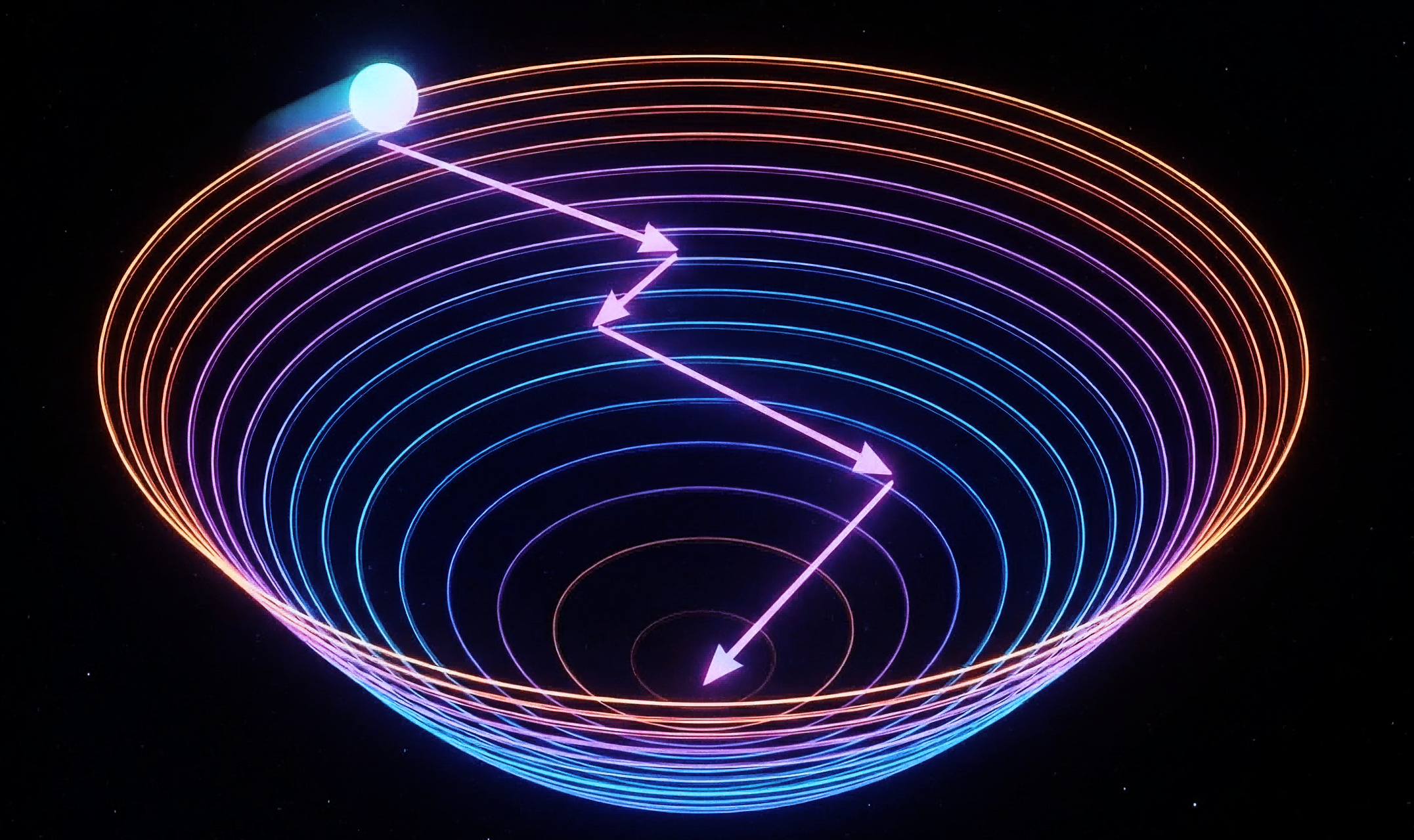
Imagine standing on a hilly landscape in thick fog. The goal is to reach the lowest point (minimum loss), but visibility is limited to just the immediate surroundings. The strategy? Feel the slope under your feet and step downhill. Repeat until flat ground is reached.

This is exactly what gradient descent does mathematically:

1. Calculate the slope (gradient) at the current position
2. Take a step in the direction of steepest descent
3. Repeat until convergence

The Optimization Problem

Given a loss function $J(w)$ that measures how “wrong” the model is, the goal is to find the optimal weights:

$$w^* = \arg\min_w J(w)$$

For most ML problems, $J(w)$ is a complex function of many parameters. Finding the exact minimum analytically is often impossible. Gradient descent provides an iterative numerical solution.

The Gradient: Which Way is Downhill?

The gradient $\nabla J(w)$ is a vector that points in the direction of steepest ascent — the direction where the function increases fastest.

For a function of multiple variables $J(w_1, w_2, …, w_n)$:

$$\nabla J(w) = \begin{bmatrix} \frac{\partial J}{\partial w_1} \ \frac{\partial J}{\partial w_2} \ \vdots \ \frac{\partial J}{\partial w_n} \end{bmatrix}$$

Key insight: To minimize the function, move in the opposite direction of the gradient — the direction of steepest descent.

The Update Rule

The gradient descent update is elegantly simple:

$$w_{t+1} = w_t - \eta \nabla J(w_t)$$

Where:

• $w_t$ = current parameter values
• $\eta$ = learning rate (step size)
• $\nabla J(w_t)$ = gradient at current position
• $w_{t+1}$ = new parameter values

Understanding the Learning Rate

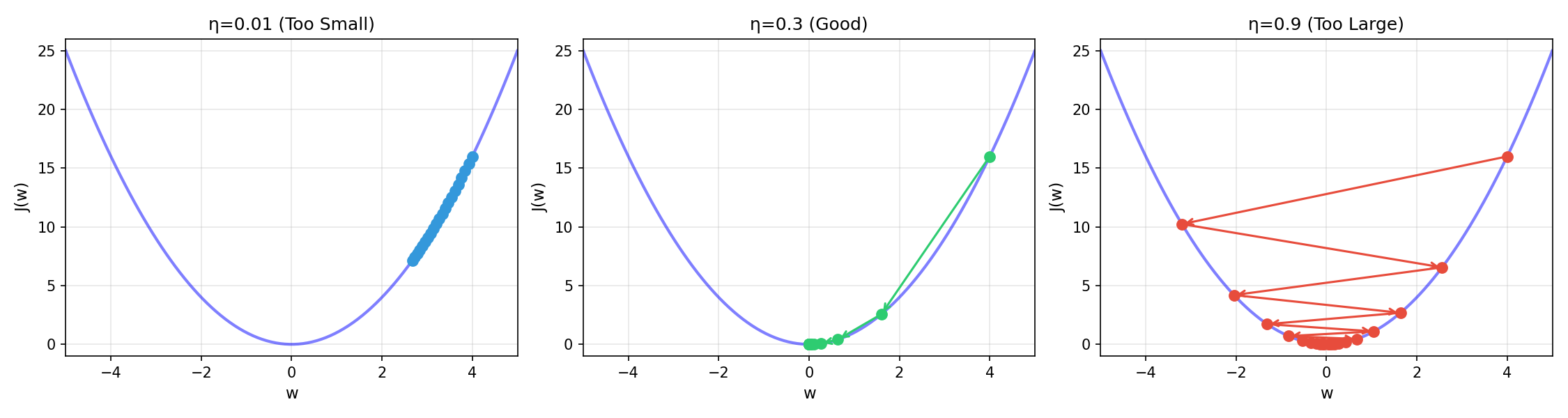
The learning rate $\eta$ controls how big each step is. This single hyperparameter dramatically affects training behavior:

Practical guidelines for choosing $\eta$:

• Start with common values: 0.01, 0.001, or 0.0001
• If loss decreases too slowly → increase $\eta$
• If loss oscillates or increases → decrease $\eta$
• Consider learning rate schedules that reduce $\eta$ over time

Convergence: When to Stop?

Gradient descent continues until one of these stopping criteria is met:

Batch Gradient Descent vs. Stochastic Gradient Descent

The standard gradient descent formula uses all training samples to compute the gradient:

$$\nabla J(w) = \frac{1}{N} \sum_{i=1}^{N} \nabla L(w; x_i, y_i)$$

This is called Batch Gradient Descent (BGD). It’s accurate but slow for large datasets.

Stochastic Gradient Descent (SGD) uses only one random sample per update:

$$\nabla J(w) \approx \nabla L(w; x_i, y_i)$$

Mini-batch GD is the compromise — use a small batch of samples (typically 32-256):

$$\nabla J(w) \approx \frac{1}{B} \sum_{i=1}^{B} \nabla L(w; x_i, y_i)$$

Why does SGD work despite noisy gradients?

The noise in SGD gradients acts as implicit regularization — it helps escape local minima and can lead to better generalization. The key insight is that while each individual update may be inaccurate, the average direction over many updates still points toward the minimum.

The Loss Landscape Perspective

Visualizing the loss function as a landscape helps build intuition:

• Convex functions (like linear/logistic regression loss): One global minimum, gradient descent always converges
• Non-convex functions (like neural networks): Multiple local minima and saddle points, convergence depends on initialization and learning rate

Code Practice

This section demonstrates gradient descent through interactive visualizations and practical implementations.

Learning Rate Comparison

The following code visualizes how different learning rates affect convergence:

 1
 2
 3
 4
 5
 6
 7
 8
 9
10
11
12
13
14
15
16
17
18
19
20
21
22
23
24
25
26
27
28
29
30
31
32
33
34
35
36
37
38
39
40
41
42
43
44
45
46
47

import numpy as np
import matplotlib.pyplot as plt

# Loss function: J(w) = w^2 (minimum at w=0)
def J(w): return w**2
def grad_J(w): return 2*w

def gradient_descent(w0, lr, steps):
    """Run gradient descent and return history."""
    w = w0
    history = [w]
    for _ in range(steps):
        w = w - lr * grad_J(w)
        history.append(w)
    return history

# Compare three learning rates
learning_rates = [0.01, 0.3, 0.9]
labels = ['η=0.01 (Too Small)', 'η=0.3 (Good)', 'η=0.9 (Too Large)']
colors = ['#3498db', '#2ecc71', '#e74c3c']

fig, axes = plt.subplots(1, 3, figsize=(15, 4))
w_range = np.linspace(-5, 5, 100)

for ax, lr, label, color in zip(axes, learning_rates, labels, colors):
    history = gradient_descent(w0=4.0, lr=lr, steps=20)
    
    # Plot loss curve
    ax.plot(w_range, J(w_range), 'b-', alpha=0.5, linewidth=2)
    
    # Plot gradient descent path
    for i in range(len(history)-1):
        ax.annotate('', xy=(history[i+1], J(history[i+1])),
                   xytext=(history[i], J(history[i])),
                   arrowprops=dict(arrowstyle='->', color=color, lw=1.5))
    ax.scatter(history, [J(w) for w in history], c=color, s=50, zorder=5)
    
    ax.set_xlabel('w', fontsize=11)
    ax.set_ylabel('J(w)', fontsize=11)
    ax.set_title(label, fontsize=12)
    ax.set_xlim(-5, 5)
    ax.set_ylim(-1, 26)
    ax.grid(alpha=0.3)

plt.tight_layout()
plt.savefig('assets/learning_rate_comparison.png', dpi=150)
plt.show()

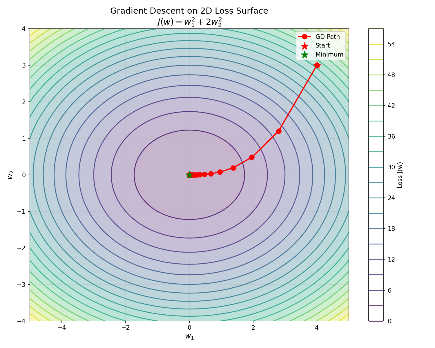
2D Contour Plot: Gradient Descent Path

Visualizing gradient descent on a 2D loss surface provides deeper intuition:

 1
 2
 3
 4
 5
 6
 7
 8
 9
10
11
12
13
14
15
16
17
18
19
20
21
22
23
24
25
26
27
28
29
30
31
32
33
34
35
36
37
38
39
40
41
42
43
44
45
46

import numpy as np
import matplotlib.pyplot as plt

# 2D loss function: J(w1, w2) = w1^2 + 2*w2^2 (elliptical bowl)
def J_2d(w1, w2): return w1**2 + 2*w2**2
def grad_J_2d(w1, w2): return np.array([2*w1, 4*w2])

# Gradient descent on 2D surface
def gd_2d(w0, lr, steps):
    w = np.array(w0, dtype=float)
    history = [w.copy()]
    for _ in range(steps):
        w = w - lr * grad_J_2d(w[0], w[1])
        history.append(w.copy())
    return np.array(history)

# Run gradient descent
history = gd_2d(w0=[4.0, 3.0], lr=0.15, steps=30)

# Create contour plot
fig, ax = plt.subplots(figsize=(10, 8))

w1_range = np.linspace(-5, 5, 100)
w2_range = np.linspace(-4, 4, 100)
W1, W2 = np.meshgrid(w1_range, w2_range)
Z = J_2d(W1, W2)

# Contour plot
contour = ax.contour(W1, W2, Z, levels=20, cmap='viridis', alpha=0.8)
ax.contourf(W1, W2, Z, levels=20, cmap='viridis', alpha=0.3)
plt.colorbar(contour, label='Loss J(w)')

# Gradient descent path
ax.plot(history[:, 0], history[:, 1], 'ro-', markersize=8, linewidth=2, label='GD Path')
ax.scatter(history[0, 0], history[0, 1], c='red', s=150, marker='*', zorder=5, label='Start')
ax.scatter(0, 0, c='green', s=150, marker='*', zorder=5, label='Minimum')

ax.set_xlabel('$w_1$', fontsize=12)
ax.set_ylabel('$w_2$', fontsize=12)
ax.set_title('Gradient Descent on 2D Loss Surface\n$J(w) = w_1^2 + 2w_2^2$', fontsize=14)
ax.legend()
ax.grid(alpha=0.3)

plt.tight_layout()
plt.savefig('assets/loss_landscape.png', dpi=150)
plt.show()

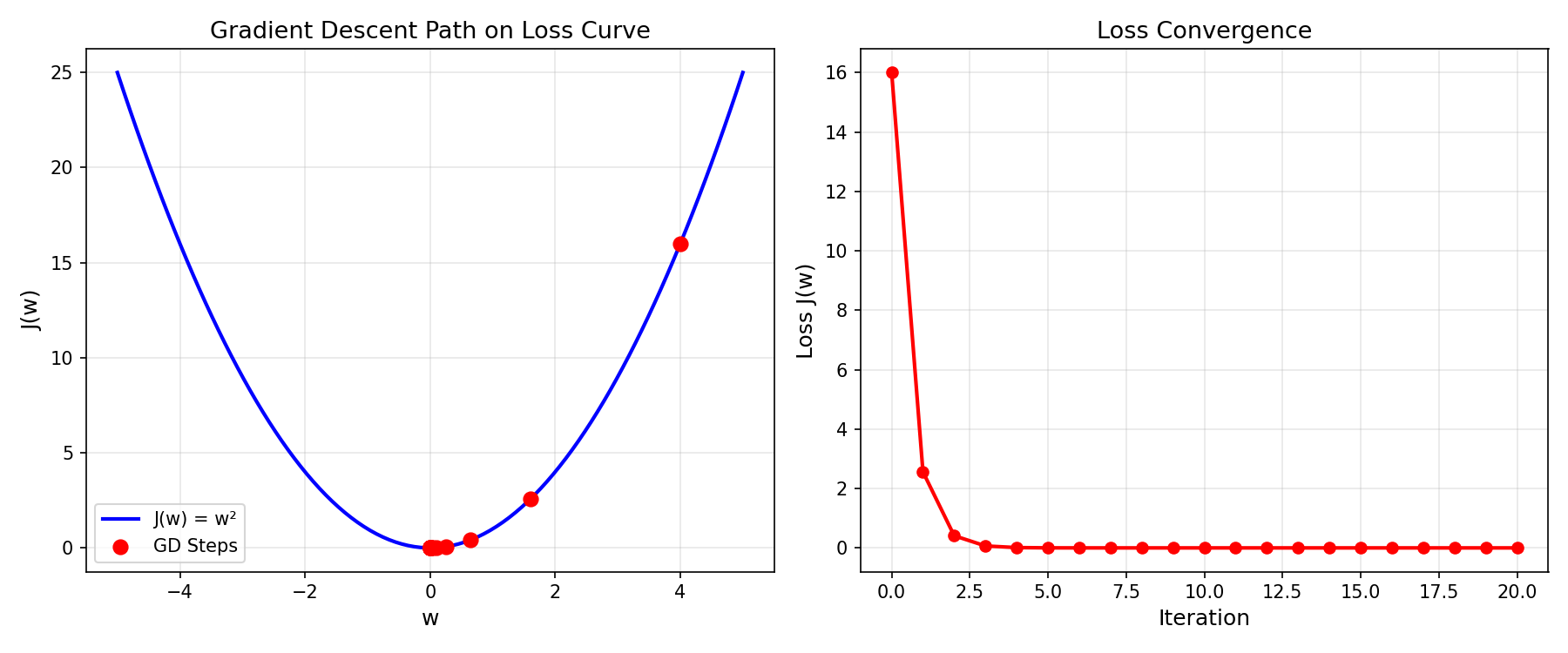
Gradient Descent on a Simple Parabola

 1
 2
 3
 4
 5
 6
 7
 8
 9
10
11
12
13
14
15
16
17
18
19
20
21
22
23
24
25
26
27
28
29
30
31
32
33
34
35
36
37
38
39
40
41

import numpy as np
import matplotlib.pyplot as plt

# Simple quadratic: J(w) = w^2
def J(w): return w**2
def grad_J(w): return 2*w

# Gradient descent
w = 4.0
lr = 0.3
history = [w]
losses = [J(w)]

for _ in range(20):
    w = w - lr * grad_J(w)
    history.append(w)
    losses.append(J(w))

# Plot
fig, (ax1, ax2) = plt.subplots(1, 2, figsize=(12, 5))

# Left: GD path on loss curve
w_range = np.linspace(-5, 5, 100)
ax1.plot(w_range, J(w_range), 'b-', linewidth=2, label='J(w) = w²')
ax1.scatter(history, [J(w) for w in history], c='red', s=60, zorder=5, label='GD Steps')
ax1.set_xlabel('w', fontsize=12)
ax1.set_ylabel('J(w)', fontsize=12)
ax1.set_title('Gradient Descent Path on Loss Curve', fontsize=13)
ax1.legend()
ax1.grid(alpha=0.3)

# Right: Loss over iterations
ax2.plot(range(len(losses)), losses, 'ro-', linewidth=2, markersize=6)
ax2.set_xlabel('Iteration', fontsize=12)
ax2.set_ylabel('Loss J(w)', fontsize=12)
ax2.set_title('Loss Convergence', fontsize=13)
ax2.grid(alpha=0.3)

plt.tight_layout()
plt.savefig('assets/gd_convergence.png', dpi=150)
plt.show()

Logistic Regression with Gradient Descent

🐍 Python

1 2 3 4 5 6 7 8 9 10 11 12 13 14 15 16 17 18 19 20 21 22 23 24 25 26 27 28

def logistic_regression_gd(X, y, lr=0.1, epochs=1000): X_b = np.c_[np.ones(len(X)), X] w = np.zeros(X_b.shape[1]) losses = [] for _ in range(epochs): z = X_b @ w y_pred = 1 / (1 + np.exp(-z)) # Cross-entropy loss loss = -np.mean(y * np.log(y_pred + 1e-8) + (1-y) * np.log(1-y_pred + 1e-8)) losses.append(loss) # Gradient gradient = X_b.T @ (y_pred - y) / len(y) w -= lr * gradient return w, losses # Example from sklearn.datasets import make_classification X, y = make_classification(n_samples=200, n_features=2, n_redundant=0, random_state=42) w, losses = logistic_regression_gd(X, y, lr=0.5, epochs=100) plt.plot(losses) plt.xlabel('Epoch'); plt.ylabel('Loss') plt.title('Training Loss') plt.savefig('assets/loss_curve.png')

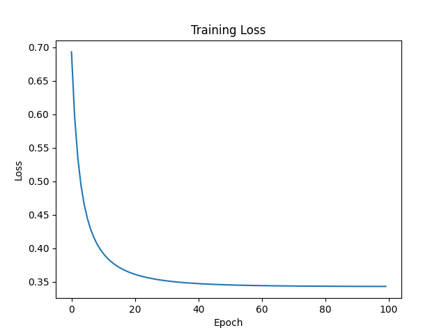
SGD Implementation

 1
 2
 3
 4
 5
 6
 7
 8
 9
10
11
12
13
14
15
16
17
18
19
20

def logistic_regression_sgd(X, y, lr=0.01, epochs=50):
    X_b = np.c_[np.ones(len(X)), X]
    w = np.zeros(X_b.shape[1])
    
    for epoch in range(epochs):
        # Shuffle data each epoch
        indices = np.random.permutation(len(X))
        
        for i in indices:
            xi = X_b[i:i+1]
            yi = y[i:i+1]
            
            y_pred = 1 / (1 + np.exp(-xi @ w))
            gradient = xi.T @ (y_pred - yi)
            w -= lr * gradient.ravel()
    
    return w

w_sgd = logistic_regression_sgd(X, y, lr=0.1, epochs=20)
print(f"SGD weights: {w_sgd}")

Output:

1

SGD weights: [-0.12936055  2.39858137 -0.10648485]

Comparing GD vs SGD

 1
 2
 3
 4
 5
 6
 7
 8
 9
10

from sklearn.linear_model import SGDClassifier, LogisticRegression

# Batch (full GD via solver)
clf_batch = LogisticRegression(solver='lbfgs').fit(X, y)

# SGD
clf_sgd = SGDClassifier(loss='log_loss', max_iter=1000).fit(X, y)

print(f"Batch accuracy: {clf_batch.score(X, y):.2%}")
print(f"SGD accuracy: {clf_sgd.score(X, y):.2%}")

Output:

1
2

Batch accuracy: 86.50%
SGD accuracy: 84.50%

Deep Dive

This section addresses common questions and introduces advanced optimization techniques.

Q1: How to choose the right learning rate?

Finding the optimal learning rate is one of the most important hyperparameter decisions. Practical approaches include:

Q2: When to use SGD vs. batch GD?

Q3: What mini-batch size should be used?

Note: Powers of 2 (32, 64, 128, 256) are GPU-friendly due to memory alignment.

Advanced Optimizers

While basic gradient descent works, modern ML uses adaptive optimizers that automatically adjust learning rates:

Momentum

Standard GD can oscillate in ravines (narrow valleys). Momentum adds “velocity” to smooth out oscillations:

$$v_t = \gamma v_{t-1} + \eta \nabla J(w_t)$$ $$w_{t+1} = w_t - v_t$$

Where $\gamma \approx 0.9$ is the momentum coefficient. This accelerates convergence and dampens oscillations.

RMSprop

RMSprop adapts learning rates per-parameter based on recent gradient magnitudes:

$$E[g^2]_t = \gamma E[g^2]_{t-1} + (1-\gamma) g_t^2$$ $$w_{t+1} = w_t - \frac{\eta}{\sqrt{E[g^2]_t + \epsilon}} g_t$$

This helps with sparse features and prevents the learning rate from becoming too small.

Adam (Adaptive Moment Estimation)

Adam combines the best of Momentum and RMSprop — it’s the most popular optimizer for deep learning:

$$m_t = \beta_1 m_{t-1} + (1-\beta_1) g_t \quad \text{(first moment)}$$ $$v_t = \beta_2 v_{t-1} + (1-\beta_2) g_t^2 \quad \text{(second moment)}$$ $$w_{t+1} = w_t - \frac{\eta}{\sqrt{\hat{v}_t} + \epsilon} \hat{m}_t$$

Default hyperparameters: $\beta_1 = 0.9$, $\beta_2 = 0.999$, $\epsilon = 10^{-8}$

 1
 2
 3
 4
 5
 6
 7
 8
 9
10
11

# Using optimizers in PyTorch
import torch.optim as optim

# SGD with momentum
optimizer = optim.SGD(model.parameters(), lr=0.01, momentum=0.9)

# Adam (most common choice)
optimizer = optim.Adam(model.parameters(), lr=0.001)

# RMSprop
optimizer = optim.RMSprop(model.parameters(), lr=0.01)

Learning Rate Schedules

Keeping $\eta$ constant throughout training may not be optimal. Learning rate schedules reduce $\eta$ over time:

1
2
3
4
5
6
7
8

# Learning rate scheduler in PyTorch
from torch.optim.lr_scheduler import StepLR, CosineAnnealingLR

# Reduce LR by 0.1 every 10 epochs
scheduler = StepLR(optimizer, step_size=10, gamma=0.1)

# Cosine annealing
scheduler = CosineAnnealingLR(optimizer, T_max=100)

Summary

Key Formulas

Key Takeaways

1. Gradient descent minimizes loss iteratively — no closed-form solution needed
2. Learning rate is critical — too small is slow, too large diverges
3. SGD trades accuracy for speed — noisy gradients but faster updates
4. Mini-batch balances the trade-off — typical sizes: 32-256
5. Adaptive optimizers (Adam) often work best — automatically adjust learning rates
6. Learning rate schedules improve convergence — reduce $\eta$ over time

Practical Recommendations

References

• Bottou, L. (2010). “Large-Scale Machine Learning with Stochastic Gradient Descent”
• Kingma, D. & Ba, J. (2014). “Adam: A Method for Stochastic Optimization”
• Ruder, S. (2016). “An Overview of Gradient Descent Optimization Algorithms”
• sklearn SGD Classifier
• PyTorch Optimizers