Learning Objectives

• Understand the maximum margin intuition
• Formulate the hard-margin optimization problem
• Identify support vectors
• Grasp the dual problem basics

Theory

What is SVM?

Support Vector Machine (SVM) is a supervised learning algorithm for classification and regression tasks. First introduced by Vapnik and colleagues in the 1990s, SVM remains one of the most powerful and widely-used classifiers in machine learning.

The core idea: find the optimal hyperplane that separates different classes with the maximum margin. Unlike other classifiers that simply find any separating boundary, SVM seeks the boundary that is most robust to new data.

Why Maximize Margin?

When separating two groups of points, infinitely many lines can achieve perfect classification — but which one is best?

Key insight: A classifier with a larger margin is more robust and generalizes better. The margin acts as a “safety buffer” — the wider it is, the higher the confidence that new, unseen points will be classified correctly.

A small margin means even tiny perturbations in data could cause misclassification. A large margin provides robustness against noise and improves generalization to new data.

Hyperplane Geometry

A hyperplane in $\mathbb{R}^n$ is defined by:

$$w^T x + b = 0$$

where:

• $w \in \mathbb{R}^n$ is the normal vector (perpendicular to the hyperplane)
• $b \in \mathbb{R}$ is the bias (shifts the hyperplane from the origin)

Distance from a Point to Hyperplane

For any point $x_0$, the signed distance to the hyperplane is:

$$\text{distance} = \frac{w^T x_0 + b}{|w|}$$

For a correctly classified point with label $y_i \in {-1, +1}$:

$$\text{functional margin} = y_i(w^T x_i + b)$$

$$\text{geometric margin} = \frac{y_i(w^T x_i + b)}{|w|}$$

The geometric margin is the actual Euclidean distance, invariant to scaling of $w$ and $b$.

From Margin to Optimization

Goal: Find the hyperplane that maximizes the minimum geometric margin.

Step 1: Define the Margin

The margin of the classifier is the distance to the nearest point:

$$\gamma = \min_i \frac{y_i(w^T x_i + b)}{|w|}$$

Step 2: Normalize the Constraints

Since scaling $w$ and $b$ produces the same hyperplane, this freedom can be fixed by requiring that for the closest points:

$$y_i(w^T x_i + b) = 1 \quad \text{(for support vectors)}$$

This means all other points satisfy:

$$y_i(w^T x_i + b) \geq 1$$

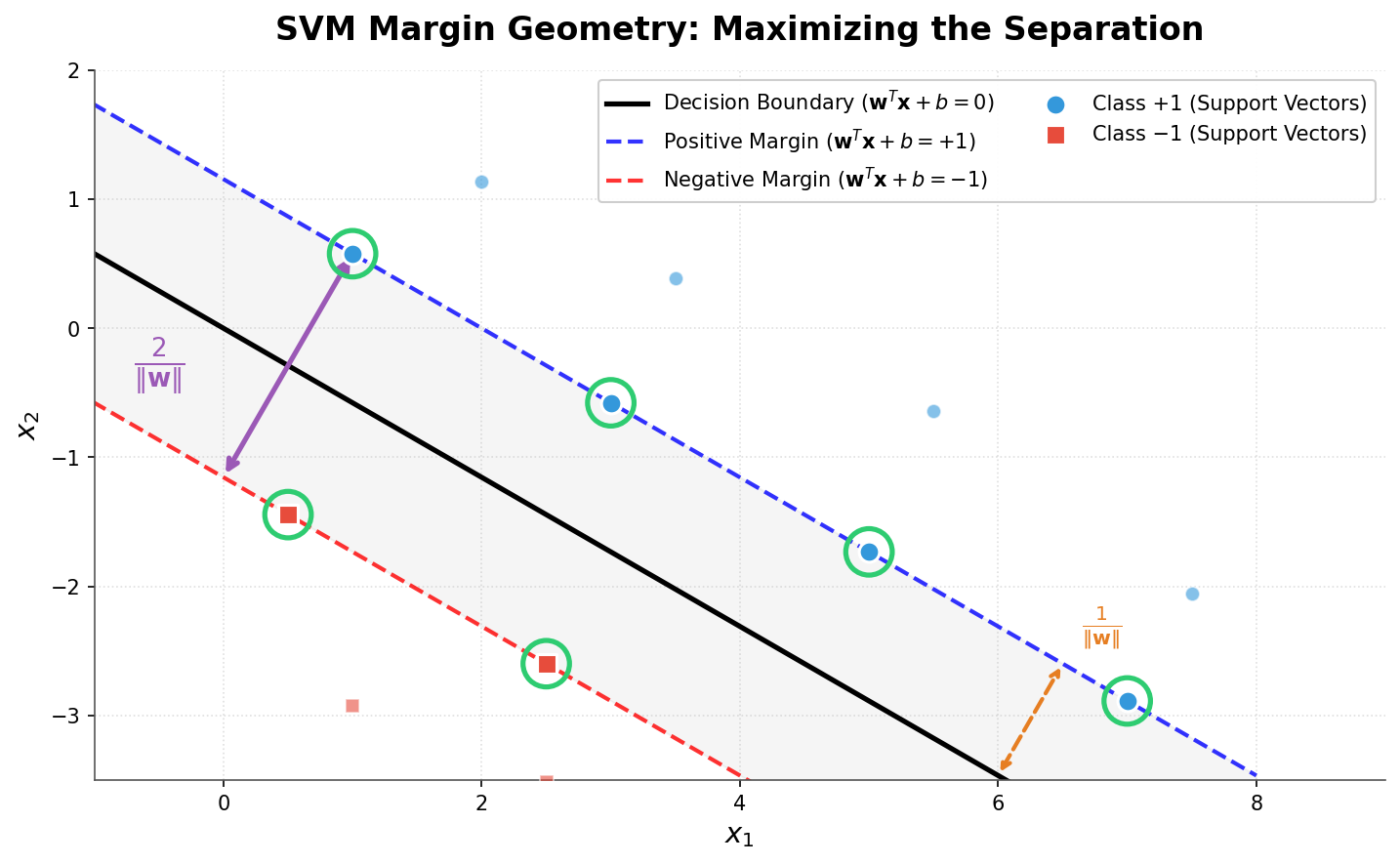
With this normalization, the geometric margin of the closest points becomes:

$$\gamma = \frac{1}{|w|}$$

Step 3: Formulate the Optimization Problem

Maximize margin → Maximize $\dfrac{1}{|w|}$ → Minimize $|w|$ → Minimize $\dfrac{1}{2}|w|^2$

The Hard-Margin SVM Primal Problem:

$$\boxed{\min_{w,b} \frac{1}{2}|w|^2 \quad \text{s.t.} \quad y_i(w^T x_i + b) \geq 1, ; \forall i = 1, \ldots, N}$$

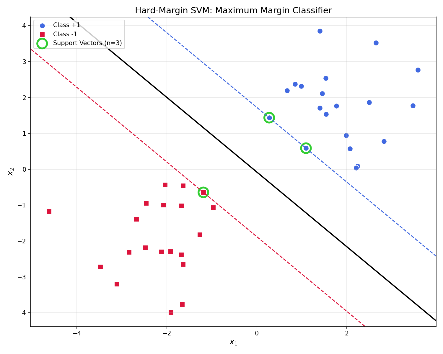
Support Vectors

Support vectors are the critical data points that lie exactly on the margin boundary:

$$y_i(w^T x_i + b) = 1$$

Key properties:

• They are the closest points to the decision boundary
• They fully determine the hyperplane — remove other points and the solution doesn’t change
• Typically only a small subset of training points are support vectors

Lagrangian and KKT Conditions

To solve the constrained optimization problem, Lagrange multipliers are introduced.

The Lagrangian

Introduce multipliers $\alpha_i \geq 0$ for each constraint:

$$\mathcal{L}(w, b, \alpha) = \frac{1}{2}|w|^2 - \sum_{i=1}^{N} \alpha_i \left[ y_i(w^T x_i + b) - 1 \right]$$

The primal problem becomes:

$$\min_{w,b} \max_{\alpha \geq 0} \mathcal{L}(w, b, \alpha)$$

KKT Conditions (Intuitive View)

The Karush-Kuhn-Tucker (KKT) conditions are necessary and sufficient for optimality:

Deriving the Dual Problem

The KKT conditions provide a path to solve for $w$ and $b$.

Step 1: Differentiate and Set to Zero

$$\frac{\partial \mathcal{L}}{\partial w} = w - \sum_{i=1}^{N} \alpha_i y_i x_i = 0 \quad \Rightarrow \quad \boxed{w = \sum_{i=1}^{N} \alpha_i y_i x_i}$$

$$\frac{\partial \mathcal{L}}{\partial b} = -\sum_{i=1}^{N} \alpha_i y_i = 0 \quad \Rightarrow \quad \boxed{\sum_{i=1}^{N} \alpha_i y_i = 0}$$

Step 2: Substitute Back into Lagrangian

Substituting $w = \sum_i \alpha_i y_i x_i$ into $\mathcal{L}$:

$$\mathcal{L} = \frac{1}{2} \left| \sum_i \alpha_i y_i x_i \right|^2 - \sum_i \alpha_i y_i \left( \sum_j \alpha_j y_j x_j \right)^T x_i - b\sum_i \alpha_i y_i + \sum_i \alpha_i$$

Since $\sum_i \alpha_i y_i = 0$, the $b$ term vanishes. After simplification:

$$\mathcal{L} = \sum_i \alpha_i - \frac{1}{2} \sum_{i,j} \alpha_i \alpha_j y_i y_j x_i^T x_j$$

Step 3: The Dual Problem

The Hard-Margin SVM Dual Problem:

$$\boxed{\begin{aligned} \max_\alpha \quad & \sum_{i=1}^{N} \alpha_i - \frac{1}{2} \sum_{i,j} \alpha_i \alpha_j y_i y_j (x_i^T x_j) \\ \text{s.t.} \quad & \alpha_i \geq 0, ; \forall i \\ & \sum_{i=1}^{N} \alpha_i y_i = 0 \end{aligned}}$$

Why the Dual Matters

The dual formulation has several crucial advantages:

Code Practice

The following examples demonstrate Hard-Margin SVM implementation and visualization of the optimal separating hyperplane.

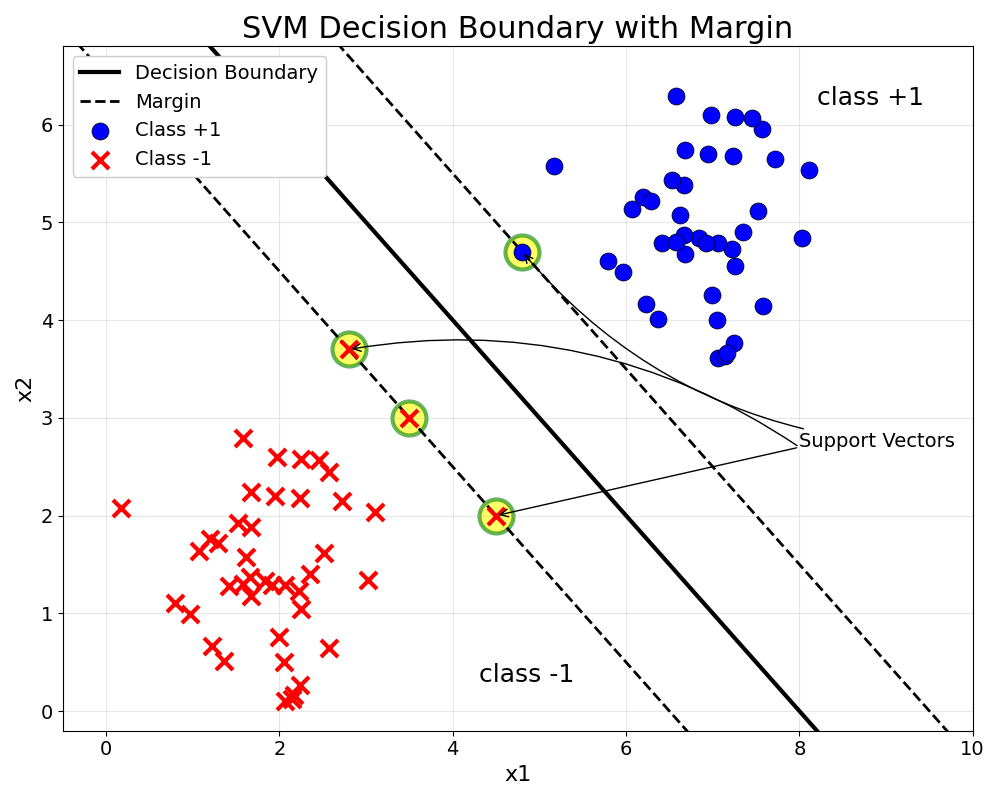
Hard-Margin SVM Visualization

This example generates linearly separable data and trains an SVM with a very large C value (regularization parameter) to simulate hard-margin behavior. A large C means the model strongly penalizes any misclassification, effectively enforcing hard constraints.

 1
 2
 3
 4
 5
 6
 7
 8
 9
10
11
12
13
14
15
16
17
18
19
20
21
22
23
24
25
26
27
28
29
30
31
32
33
34
35
36
37
38
39
40
41
42
43
44
45
46
47
48
49
50
51
52
53
54

import numpy as np
import matplotlib.pyplot as plt
from sklearn.svm import SVC

# Generate linearly separable data
np.random.seed(42)
X = np.vstack([
    np.random.randn(20, 2) + [2, 2],    # Class +1: centered at (2, 2)
    np.random.randn(20, 2) + [-2, -2]   # Class -1: centered at (-2, -2)
])
y = np.array([1]*20 + [-1]*20)

# Train hard-margin SVM
# C=1e10 simulates hard margin (infinite penalty for misclassification)
svm = SVC(kernel='linear', C=1e10)
svm.fit(X, y)

# Create visualization
plt.figure(figsize=(10, 8))
plt.scatter(X[y==1][:, 0], X[y==1][:, 1], c='royalblue', marker='o', 
            s=80, label='Class +1', edgecolors='white')
plt.scatter(X[y==-1][:, 0], X[y==-1][:, 1], c='crimson', marker='s', 
            s=80, label='Class -1', edgecolors='white')

# Plot decision boundary and margins
ax = plt.gca()
xlim = ax.get_xlim()
ylim = ax.get_ylim()

xx = np.linspace(xlim[0], xlim[1], 100)
yy = np.linspace(ylim[0], ylim[1], 100)
YY, XX = np.meshgrid(yy, xx)
xy = np.vstack([XX.ravel(), YY.ravel()]).T
Z = svm.decision_function(xy).reshape(XX.shape)

# Decision boundary (Z=0) and margin lines (Z=-1, Z=+1)
ax.contour(XX, YY, Z, levels=[-1, 0, 1], 
           linestyles=['--', '-', '--'], 
           colors=['crimson', 'black', 'royalblue'],
           linewidths=[1.5, 2, 1.5])

# Highlight support vectors with larger circles
ax.scatter(svm.support_vectors_[:, 0], svm.support_vectors_[:, 1],
           s=250, facecolors='none', edgecolors='limegreen', linewidths=3,
           label=f'Support Vectors (n={len(svm.support_vectors_)})')

plt.legend(loc='upper left')
plt.xlabel('$x_1$', fontsize=12)
plt.ylabel('$x_2$', fontsize=12)
plt.title('Hard-Margin SVM: Maximum Margin Classifier', fontsize=14)
plt.grid(True, alpha=0.3)
plt.tight_layout()
plt.savefig('assets/svm_margin.png', dpi=150)
plt.show()

Output:

The solid black line is the decision boundary ($w^Tx + b = 0$). The dashed lines show the margin boundaries where $w^Tx + b = \pm 1$. Points circled in green are the support vectors — notice how they lie exactly on the margin boundaries.

Examining Support Vectors

The following code inspects the learned model parameters and verifies the margin calculation.

 1
 2
 3
 4
 5
 6
 7
 8
 9
10
11
12
13
14
15
16
17
18
19
20
21
22
23
24
25
26
27
28

# Model parameters
print("=" * 50)
print("SVM MODEL ANALYSIS")
print("=" * 50)

print(f"\n📊 Support Vectors:")
print(f"   Count: {len(svm.support_vectors_)}")
print(f"   Indices: {svm.support_}")
print(f"   Per class: {svm.n_support_}")

print(f"\n⚖️ Hyperplane Parameters:")
print(f"   Weights (w): [{svm.coef_[0][0]:.4f}, {svm.coef_[0][1]:.4f}]")
print(f"   Bias (b): {svm.intercept_[0]:.4f}")

# Compute margin width
w = svm.coef_[0]
w_norm = np.linalg.norm(w)
margin_width = 2 / w_norm

print(f"\n📏 Margin Analysis:")
print(f"   ||w|| = {w_norm:.4f}")
print(f"   Margin width (2/||w||) = {margin_width:.4f}")

# Verify support vectors lie on margin
print(f"\n✅ Verification (SVs should have |decision| = 1):")
for i, sv in enumerate(svm.support_vectors_[:3]):  # Show first 3
    decision = svm.decision_function([sv])[0]
    print(f"   SV {i+1}: decision_function = {decision:.6f}")

Output:

 1
 2
 3
 4
 5
 6
 7
 8
 9
10
11
12
13
14
15
16
17
18
19
20
21

==================================================
SVM MODEL ANALYSIS
==================================================

📊 Support Vectors:
   Count: 3
   Indices: [32  7  9]
   Per class: [1 2]

⚖️ Hyperplane Parameters:
   Weights (w): [0.5778, 0.5553]
   Bias (b): 0.0430

📏 Margin Analysis:
   ||w|| = 0.8014
   Margin width (2/||w||) = 2.4958

✅ Verification (SVs should have |decision| = 1):
   SV 1: decision_function = -1.000558
   SV 2: decision_function = 1.000279
   SV 3: decision_function = 1.000279

Using sklearn SVM in Practice

The following example presents a more realistic scenario with train/test split and accuracy evaluation.

 1
 2
 3
 4
 5
 6
 7
 8
 9
10
11
12
13
14
15
16
17
18
19
20
21
22
23
24
25
26
27
28
29
30
31
32

from sklearn.datasets import make_classification
from sklearn.model_selection import train_test_split
from sklearn.preprocessing import StandardScaler

# Generate a classification dataset
X, y = make_classification(n_samples=200, n_features=2, n_redundant=0,
                           n_informative=2, n_clusters_per_class=1, 
                           class_sep=2.0, random_state=42)
y = np.where(y == 0, -1, 1)  # Convert to {-1, +1}

# Split and scale
X_train, X_test, y_train, y_test = train_test_split(
    X, y, test_size=0.2, random_state=42
)
scaler = StandardScaler()
X_train_scaled = scaler.fit_transform(X_train)
X_test_scaled = scaler.transform(X_test)

# Train SVM (large C for near-hard-margin)
svm = SVC(kernel='linear', C=1000)
svm.fit(X_train_scaled, y_train)

# Evaluate
train_acc = svm.score(X_train_scaled, y_train)
test_acc = svm.score(X_test_scaled, y_test)
sv_ratio = len(svm.support_vectors_) / len(X_train)

print(f"📈 Performance Metrics:")
print(f"   Train Accuracy: {train_acc:.2%}")
print(f"   Test Accuracy:  {test_acc:.2%}")
print(f"\n🎯 Model Sparsity:")
print(f"   Support Vectors: {len(svm.support_vectors_)} / {len(X_train)} ({sv_ratio:.1%})")

Output:

1
2
3
4
5
6

📈 Performance Metrics:
   Train Accuracy: 98.12%
   Test Accuracy:  97.50%

🎯 Model Sparsity:
   Support Vectors: 13 / 160 (8.1%)

Deep Dive

Frequently Asked Questions

Q1: Why does maximizing the margin improve generalization?

This connects to statistical learning theory. Intuitively:

1. Robustness: A larger margin means small perturbations (noise) in the data are less likely to cause misclassification
2. VC Dimension: Larger margins correspond to lower VC dimension, which bounds generalization error
3. Structural Risk Minimization: SVM balances empirical error (training accuracy) with model complexity (margin width)

Consider: if a decision boundary barely squeezes between two classes, any new data point slightly different from training data might fall on the wrong side. A wide margin provides a “buffer zone.”

Q2: How do support vectors fully determine the decision boundary?

From the dual solution:

$$w = \sum_{i=1}^{N} \alpha_i y_i x_i$$

Due to complementary slackness, $\alpha_i > 0$ only for support vectors. This means:

$$w = \sum_{i \in SV} \alpha_i y_i x_i$$

To find $b$, any support vector $x_s$ can be used: $$b = y_s - w^T x_s$$

Implication: All non-support-vector training points can be discarded after training — predictions rely only on SVs!

Q3: What if data is not linearly separable?

Hard-margin SVM will fail (no feasible solution exists). Two options are available:

Q4: SVM vs. Logistic Regression — When to use which?

Rule of thumb:

• Need probabilities? → Logistic Regression
• Clean separation, want robustness? → SVM
• High-dimensional data (text, genomics)? → SVM often works well

Computational Complexity

Where $N$ = number of samples, $d$ = number of features, $|SV|$ = number of support vectors.

Practical implications:

• High-dimensional data ($d \gg N$): Dual is preferred
• Many samples ($N \gg d$): Primal may be faster
• Sparse SVs: Prediction is very fast

Practical Tips

1. Check linear separability first: Plot your data. If classes clearly overlap, go straight to soft-margin or kernel SVM.

2. Monitor support vector count:

   • Too few SVs → Model might be too simple
   • Too many SVs (approaching $N$) → Data may not be separable, or C is too low

3. Start with large C, then reduce: Begin with C=1000 (near hard-margin), then decrease if overfitting.

4. Use sklearn’s dual parameter: For LinearSVC, set dual='auto' to let sklearn choose the optimal formulation.

Common Pitfalls

Summary

References

• Cortes, C. & Vapnik, V. (1995). “Support-Vector Networks”
• sklearn SVM Documentation
• Boyd, S. “Convex Optimization” - Chapter 5