ML-09: K-Nearest Neighbors (KNN)
Learning Objectives
- Understand the KNN algorithm and instance-based learning
- Master common distance metrics
- Learn how to choose the optimal K value
- Recognize the curse of dimensionality
Theory
What is K-Nearest Neighbors?
K-Nearest Neighbors (KNN) is one of the simplest and most intuitive machine learning algorithms. Unlike models that learn complex decision boundaries, KNN makes predictions based on a simple principle:
To classify a new point, find its K closest neighbors and let them vote.
graph LR
    A["❓ New Point"] --> B["Find K=3 Nearest Neighbors"]
    B --> C["🔵 Neighbor 1: Class A"]
    B --> D["🔵 Neighbor 2: Class A"]
    B --> E["🔴 Neighbor 3: Class B"]
    C --> F["🗳️ Vote: 2A vs 1B"]
    D --> F
    E --> F
    F --> G["✅ Predict: Class A"]

    style G fill:#c8e6c9
Lazy Learning vs Eager Learning
KNN is a lazy learner (also called instance-based learning):
| Aspect | Lazy Learning (KNN) | Eager Learning (Logistic Regression, SVM) |
|---|---|---|
| Training | Just store the data | Build a model from data |
| Prediction | Compute distances at query time | Use pre-built model |
| Memory | Stores entire dataset | Stores only model parameters |
| Adaptability | Easy to add new data | Need to retrain |
Distance Metrics
Since KNN relies on finding the “nearest” neighbors, how we measure distance between points is crucial. The choice of distance metric can significantly impact model performance.
Euclidean Distance (L2)
The most common metric — straight-line distance in n-dimensional space:
$$d(x, y) = \sqrt{\sum_{i=1}^{n} (x_i - y_i)^2}$$
| Example | $x$ | $y$ | Distance |
|---|---|---|---|
| 2D | (0, 0) | (3, 4) | $\sqrt{9 + 16} = 5$ |
| 3D | (1, 2, 3) | (4, 6, 3) | $\sqrt{9 + 16 + 0} = 5$ |
Manhattan Distance (L1)
Sum of absolute differences — distance along grid lines:
$$d(x, y) = \sum_{i=1}^{n} |x_i - y_i|$$
| Example | $x$ | $y$ | Distance |
|---|---|---|---|
| 2D | (0, 0) | (3, 4) | $|3| + |4| = 7$ |
Chebyshev Distance (L∞)
The maximum absolute difference across any dimension:
$$d(x, y) = \max_{i} |x_i - y_i|$$
| Example | $x$ | $y$ | Distance |
|---|---|---|---|
| 2D | (0, 0) | (3, 4) | $\max(3, 4) = 4$ |
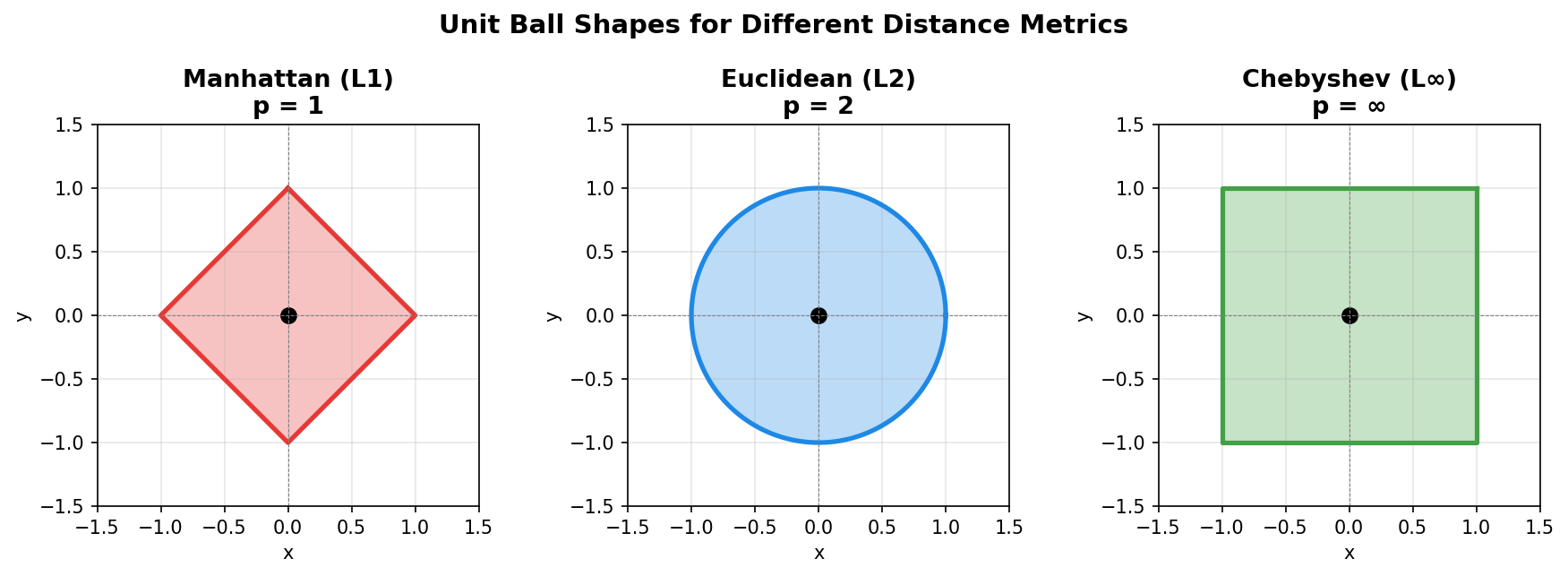
Minkowski Distance (Generalized)
Euclidean, Manhattan, and Chebyshev are all special cases of the Minkowski distance:
$$d(x, y) = \left(\sum_{i=1}^{n} |x_i - y_i|^p\right)^{1/p}$$
| $p$ | Name | Unit Ball Shape | Description |
|---|---|---|---|
| 1 | Manhattan (L1) | ◇ Diamond | Sum of absolute differences |
| 2 | Euclidean (L2) | ○ Circle | Straight-line distance |
| ∞ | Chebyshev (L∞) | □ Square | Maximum single difference |
Comparison
| Metric | Best For | Sensitivity to Outliers |
|---|---|---|
| Euclidean | Default choice, continuous features | High |
| Manhattan | High-dimensional, sparse data | Lower |
| Chebyshev | When max difference matters | Very high |
The KNN Algorithm
With distance metrics covered, the next step is to see how KNN uses them to make predictions:
Input: Training data ${(x_1, y_1), …, (x_N, y_N)}$, query point $x_q$, number of neighbors $K$
Algorithm:
- Compute distance from $x_q$ to all training points
- Sort by distance (ascending)
- Select the $K$ nearest neighbors
- Classification: Return majority class among neighbors
- Regression: Return average (or weighted average) of neighbor values
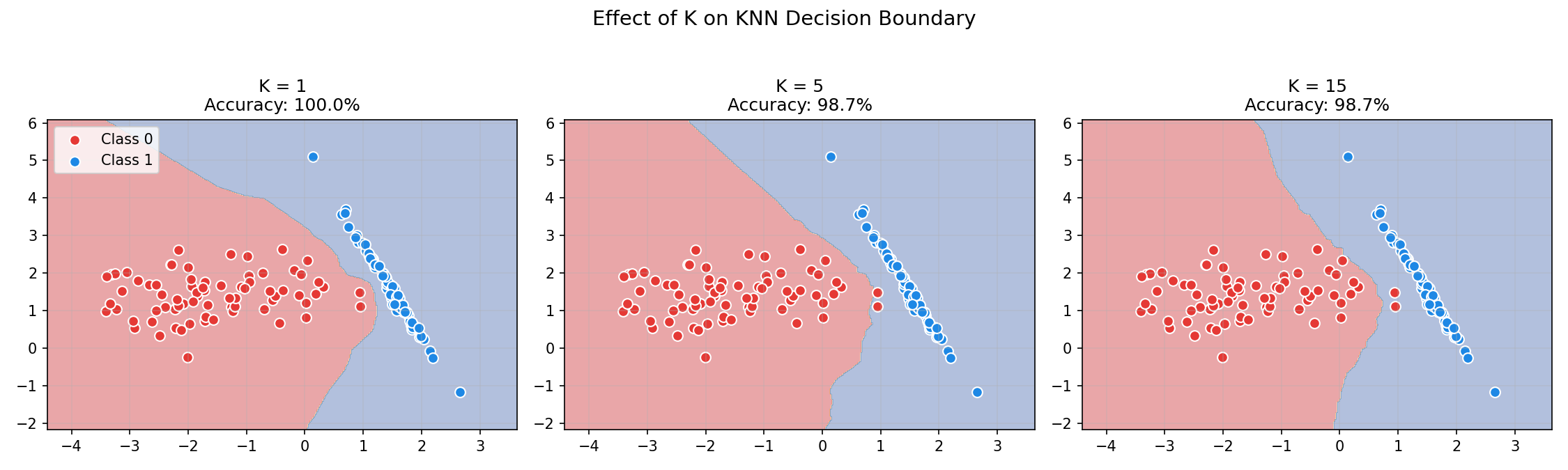
Choosing K: The Bias-Variance Tradeoff
The choice of $K$ dramatically affects model behavior:
| K Value | Behavior | Risk |
|---|---|---|
| K = 1 | Very flexible, follows training data closely | Overfitting — sensitive to noise |
| K = N | Predicts majority class for everything | Underfitting — ignores local structure |
| K = √N | Rule of thumb starting point | Balance |
Practical guidelines:
- Use odd K for binary classification (avoids ties)
- Start with $K = \sqrt{N}$ or $K = 5$
- Cross-validate to find optimal K
- Typical range: 1-20
Weighted KNN
In standard KNN, all K neighbors have equal influence on the prediction. But intuitively, closer neighbors should matter more — this is the idea behind Weighted KNN:
$$\hat{y} = \frac{\sum_{i \in N_K} w_i \cdot y_i}{\sum_{i \in N_K} w_i}$$
where $w_i = \frac{1}{d(x_q, x_i)^2}$ (inverse distance weighting)
| Method | Closer Neighbors | Farther Neighbors |
|---|---|---|
| Uniform | Same weight | Same weight |
| Distance-weighted | High weight | Low weight |
The Curse of Dimensionality
KNN works beautifully in low dimensions, but faces serious challenges as the number of features grows. This is known as the curse of dimensionality:
- Distances become meaningless: In high dimensions, all points become roughly equidistant
- Data becomes sparse: Need exponentially more data to cover the space
- Computation explodes: $O(N \cdot d)$ for each query
| Dimensions | Points needed to fill space | Nearest neighbor reliability |
|---|---|---|
| 2D | 100 | ✅ Good |
| 10D | $10^{10}$ | ⚠️ Degraded |
| 100D | $10^{100}$ | ❌ Meaningless |
Solutions:
- Reduce dimensions (PCA, t-SNE)
- Use feature selection
- Consider other algorithms for $d > 20$
Code Practice
This section implements KNN from scratch, then demonstrates sklearn for real-world applications.
KNN from Scratch
🐍 Python
| |
Output:
sklearn KNN Example
🐍 Python
| |
Output:
Finding Optimal K with Cross-Validation
🐍 Python
| |
Output:
Decision Boundary Visualization
🐍 Python
| |
Distance Metrics Comparison
🐍 Python
| |
Output:
Deep Dive
Here are answers to common questions about KNN that often come up in practice.
Frequently Asked Questions
Q1: Should I scale features before KNN?
Yes, absolutely! KNN is distance-based, so features on larger scales dominate.
| Feature Scaling | Impact on KNN |
|---|---|
| Not scaled | Features with larger range dominate distance |
| StandardScaler | Zero mean, unit variance — equal contribution |
| MinMaxScaler | [0, 1] range — also works well |
Q2: KNN vs other classifiers — when to use which?
| Scenario | Recommendation | Why |
|---|---|---|
| Small dataset, few features | KNN | Simple, effective |
| Large dataset (N > 100k) | Logistic Regression, Random Forest | KNN is too slow |
| High-dimensional (d > 20) | SVM, Random Forest | Curse of dimensionality |
| Need probability outputs | Logistic Regression | KNN probabilities are rough |
| Non-linear boundaries | KNN, SVM (RBF) | KNN handles complex shapes |
| Interpretability needed | Decision Tree | KNN is hard to explain |
Q3: How to speed up KNN?
| Method | Description | Speedup |
|---|---|---|
| KD-Tree | Tree structure for nearest neighbor search | 10-100x |
| Ball Tree | Works better in higher dimensions | 10-100x |
| Approximate NN | Trade accuracy for speed (Annoy, FAISS) | 100-1000x |
| Reduce dimensions | PCA before KNN | Depends on compression |
Q4: KNN for regression?
KNN works for regression too — just average the neighbor values:
$$\hat{y} = \frac{1}{K} \sum_{i \in N_K} y_i$$
Q5: How to handle ties in voting?
| Strategy | Description |
|---|---|
| Use odd K | For binary classification, avoids ties |
| Random selection | Pick randomly among tied classes |
| Weight by distance | Closer points break the tie |
| Increase K | Until tie is broken |
sklearn uses random selection for ties by default.
Practical Tips
KNN Checklist:
- Scale features — always!
- Start with K=5 and cross-validate
- Use odd K for binary problems
- Consider weighted voting for imbalanced data
- Check dimensions — avoid d > 20
Common Pitfalls
| Pitfall | Symptom | Solution |
|---|---|---|
| Unscaled features | Poor accuracy, one feature dominates | Use StandardScaler |
| Too small K | Overfitting, noisy predictions | Increase K |
| Too large K | Underfitting, ignores local patterns | Decrease K |
| High dimensions | Slow, poor accuracy | Reduce dimensions |
| Imbalanced classes | Predicts majority class | Use weighted KNN |
| Slow prediction | Large N or d | Use KD-tree, reduce data |
Summary
Key Formulas
| Concept | Formula |
|---|---|
| Euclidean Distance | $d(x, y) = \sqrt{\sum_i (x_i - y_i)^2}$ |
| Manhattan Distance | $d(x, y) = \sum_i |x_i - y_i|$ |
| Classification | $\hat{y} = \text{mode}(y_{N_K})$ |
| Regression | $\hat{y} = \frac{1}{K} \sum_{i \in N_K} y_i$ |
Key Takeaways
- KNN is instance-based — no training, all work at prediction time
- Distance metrics matter — Euclidean is default, Manhattan for sparse data
- K controls complexity — small K overfits, large K underfits
- Feature scaling is essential — unscaled features break KNN
- Curse of dimensionality — KNN struggles in high dimensions
- Simple but powerful — excellent baseline, competitive on small datasets
When to Use KNN
| ✅ Use When | ❌ Avoid When |
|---|---|
| Small dataset (N < 10k) | Large dataset (N > 100k) |
| Low dimensions (d < 20) | High dimensions (d > 50) |
| Non-linear patterns | Linear relationships |
| Quick baseline needed | Fast prediction required |
| Memory is available | Memory constrained |
References
- Cover, T. & Hart, P. (1967). “Nearest Neighbor Pattern Classification”
- sklearn KNeighborsClassifier
- Hastie, T. et al. “The Elements of Statistical Learning” - Chapter 13
- Beyer, K. et al. (1999). “When Is ‘Nearest Neighbor’ Meaningful?”