The k-space Pseudospectral Method: High-Speed Acoustics Simulation
Introduction
Simulating acoustic wave propagation is challenging. The domain is often large (the human body, an ocean), the medium is heterogeneous (bone, tissue, water), and the frequencies are high (MHz ultrasound). Traditional methods like Finite Difference Time Domain (FDTD) require extremely fine grids, leading to prohibitive computational costs.
Enter the k-space Pseudospectral Method—arguably the most efficient algorithm for large-scale acoustics simulation. It’s the core of the famous k-Wave Toolbox used worldwide for medical ultrasound and photoacoustic imaging research.
k-space Pseudospectral = FFT-based spatial derivatives + k-space temporal correction
This method achieves near-spectral accuracy (exponential convergence) while handling heterogeneous media like FDTD. Let’s break it down.
Prerequisites: Understanding k-space
What is k (Wavenumber)?
Just as frequency $f$ tells us “how many cycles per second,” the wavenumber $k$ tells us “how many cycles per meter”:
$$k = \frac{2\pi}{\lambda}$$
where $\lambda$ is the wavelength. Higher $k$ means shorter wavelength (finer spatial detail).
In 3D, $\mathbf{k} = (k_x, k_y, k_z)$ is a vector pointing in the wave’s propagation direction.
Physical Space vs. k-space
| Domain | Variable | Describes | Transform |
|---|---|---|---|
| Physical Space | Position $(x, y, z)$ | Where the wave is | — |
| k-space | Wavenumber $(k_x, k_y, k_z)$ | What the wave looks like (wavelength, direction) | Spatial Fourier Transform |
Key insight: k-space is to physical space what frequency domain is to time domain.
Visualization: Four Domains
Before diving into the math, let’s see what these concepts look like:
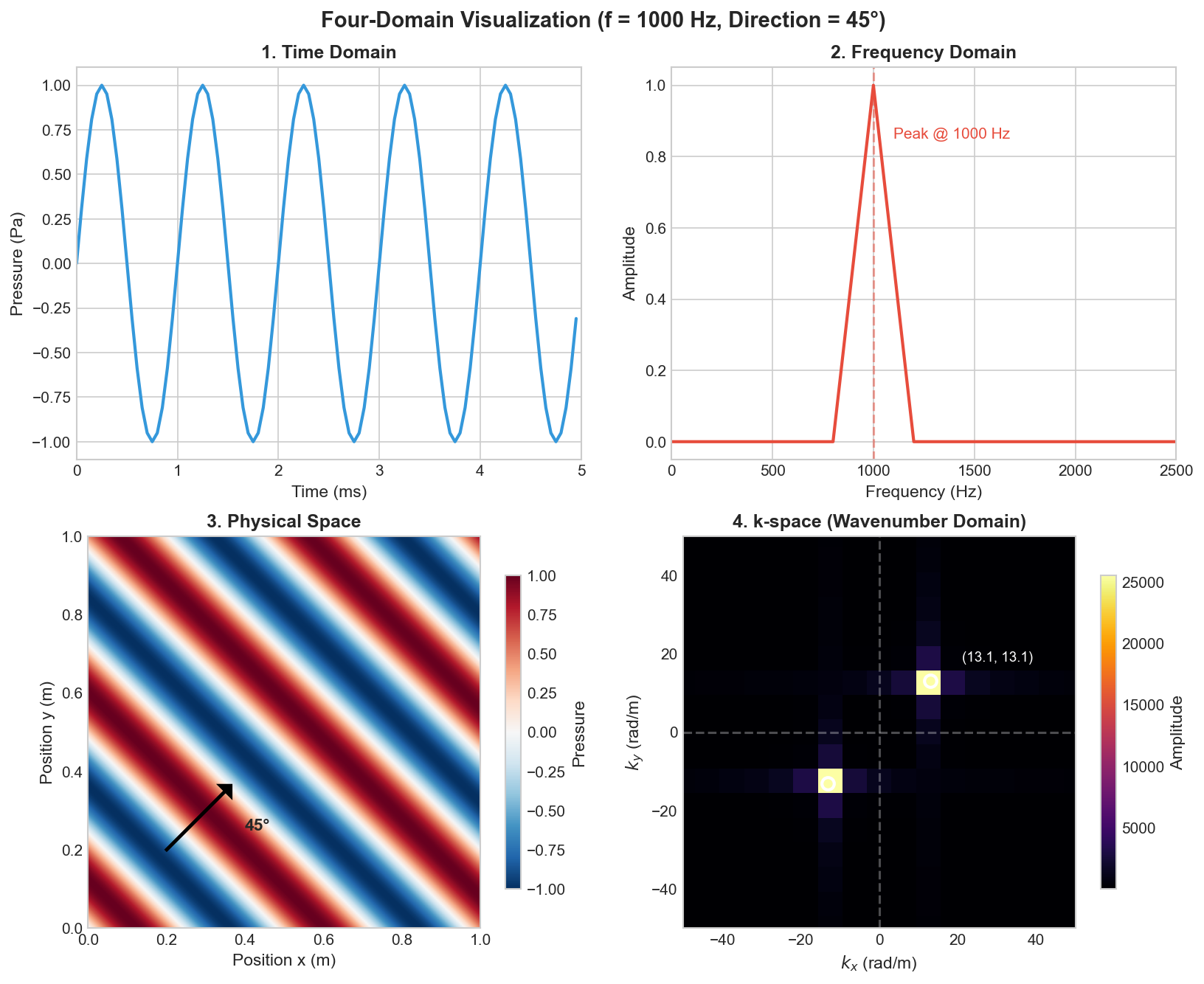
Why two points in k-space? For a real-valued signal like $\sin(k_x x + k_y y)$, the Fourier transform always produces a pair of conjugate-symmetric peaks at $(+k_x, +k_y)$ and $(-k_x, -k_y)$. This is a fundamental property: real signals have symmetric spectra. The position of these peaks tells us the wavelength (distance from origin = $|\mathbf{k}|$) and direction of propagation (angle from origin = 45°).
Why Spectral Methods Are Powerful
In spectral methods, we represent the solution as a sum of basis functions (typically Fourier modes):
$$u(x) \approx \sum_{k} \hat{u}_k e^{ikx}$$
The Magic: Differentiation Becomes Multiplication
In physical space, computing derivatives requires subtracting neighboring points (finite differences), which introduces truncation error.
In k-space, thanks to the Fourier transform property:
$$\frac{\partial}{\partial x} \quad \longrightarrow \quad \times , ik$$
Differentiation becomes simple multiplication! This eliminates numerical dispersion and achieves spectral accuracy.
flowchart LR
    A["Physical Space
u(x)"] -->|FFT| B["k-space
û(k)"]
    B -->|"×ik"| C["k-space
ik·û(k)"]
    C -->|iFFT| D["Physical Space
∂u/∂x"]
    style B fill:#e6f3ff
    style C fill:#e6f3ff
The Pseudospectral Approach
Why “Pseudo”?
Pure spectral methods work entirely in k-space. But real-world problems have spatially varying parameters like sound speed $c(x)$ in heterogeneous tissue.
The problem: Multiplying $c(x) \cdot \nabla p(x)$ in k-space requires convolution—computationally expensive.
The solution: Use k-space for what it’s good at (derivatives) and physical space for what it’s good at (multiplication).
The Pseudospectral Workflow
For each time step:
- Physical Space: Start with pressure field $p(x)$
- FFT → k-space: Transform to get $\hat{p}(k)$
- k-space: Compute gradient by multiplying by $ik$ (spectrally accurate!)
- iFFT → Physical Space: Get $\nabla p(x)$
- Physical Space: Multiply by spatially varying $c(x)^2$
- Time Update: Advance to next time step
Because we “pretend” to use spectral methods (using FFT for derivatives) but jump back to physical space for multiplication, it’s called “pseudo-spectral.”
flowchart LR
    subgraph PS["Physical Space"]
        A["p, v at time n"]
        E["Update with c²"]
        F["p, v at time n+1"]
    end
    subgraph KS["k-space"]
        B["FFT"]
        C["Multiply by ik"]
        D["iFFT"]
    end
    A --> B --> C --> D --> E --> F
    F -.-> A
    style KS fill:#fff3e6
The k-space Correction
Standard pseudospectral methods are spectrally accurate in space but still use finite differences in time (e.g., leapfrog scheme). This causes temporal dispersion—high-frequency waves travel at the wrong speed.
The k-space Operator
The k-space method introduces a Sinc-based correction:
$$\kappa = \frac{\sin(c k \Delta t / 2)}{c k \Delta t / 2}$$
This operator compensates for temporal discretization errors. For homogeneous media, the solution becomes exact regardless of time step size (within stability limits)!
Why Is This Revolutionary?
| Method | Spatial Accuracy | Temporal Accuracy | Time Step |
|---|---|---|---|
| FDTD | Low (algebraic) | Low | Very small |
| PSTD | High (spectral) | Low | Small |
| k-space PSTD | High (spectral) | High (corrected) | Larger |
Method Comparison
| Feature | FDTD | PSTD | k-space PSTD |
|---|---|---|---|
| Spatial Derivative | Neighbor subtraction | FFT | FFT |
| Temporal Scheme | Leapfrog | Leapfrog | Leapfrog + k-correction |
| Accuracy | Low (needs ~20 points/λ) | High (~π points/λ = Nyquist) | Highest |
| Heterogeneous Media | Excellent | Good | Good |
| Speed (same accuracy) | Slow | Fast | Fastest |
| Drawback | Numerical dispersion | Time step limited | Periodic boundary (needs PML) |
Applications
k-Wave Toolbox
The k-Wave toolbox (MATLAB/Python/C++) is the most popular implementation of the k-space pseudospectral method. It’s used for:
- Medical Ultrasound Simulation: Modeling wave propagation through heterogeneous tissue (bone, fat, muscle)
- Photoacoustic Imaging: Simulating initial pressure distributions converting to acoustic waves
- Therapeutic Ultrasound: High-intensity focused ultrasound (HIFU) treatment planning
Why k-space PSTD Wins
For a human body simulation at ultrasound frequencies:
- FDTD: Hundreds of millions of grid points, days of computation
- k-space PSTD: 8-10× fewer grid points, hours of computation
The only trade-off: wrap-around artifacts due to periodic FFT. This is handled by Perfectly Matched Layers (PML).
Summary
| Concept | Key Point |
|---|---|
| k-space | Spatial Fourier domain; describes wavelength and direction |
| Spectral Methods | $\partial/\partial x \to ik$; exponential accuracy |
| Pseudospectral | FFT for derivatives, physical space for multiplication |
| k-space PSTD | Adds Sinc correction for temporal accuracy |
| Result | Spectral accuracy + heterogeneous media + large time steps |
One-liner: k-space PSTD = (FFT derivatives + physical-space multiplication) + (Sinc temporal correction)
It’s the “sports car” of acoustics simulation—blazingly fast on smooth problems, with the flexibility to handle real-world heterogeneity.
References
- Treeby, B. E., & Cox, B. T. (2010). k-Wave: MATLAB toolbox for the simulation and reconstruction of photoacoustic wave fields. Journal of Biomedical Optics, 15(2), 021314.
- Tabei, M., Mast, T. D., & Waag, R. C. (2002). A k-space method for coupled first-order acoustic propagation equations. The Journal of the Acoustical Society of America, 111(1), 53-63.
- Mast, T. D., Souriau, L. P., Liu, D. L., Tabei, M., Nachman, A. I., & Waag, R. C. (2001). A k-space method for large-scale models of wave propagation in tissue. IEEE transactions on ultrasonics, ferroelectrics, and frequency control, 48(2), 341-354.