Boundary Conditions: The Key to Well-Posed Problems
Introduction
If partial differential equations are the soul of physics, then boundary conditions are the body. A beautiful equation without proper boundary conditions is like a sentence without punctuation—technically there, but meaningless or ambiguous.
Without correct boundary conditions, a PDE may have no solution, infinitely many solutions, or be physically meaningless.
Consider the steady-state heat equation $\nabla^2 T = 0$ (Laplace equation) on a metal plate. The equation tells us how temperature distributes itself at equilibrium, but it doesn’t tell us what the temperature is. Is it frozen? Boiling? That information comes from the boundaries.
The Three Classical Types
Dirichlet Boundary Condition (First Kind)
Definition: The value of the unknown function is specified on the boundary.
$$u\big|_{\partial\Omega} = g(x)$$
Physical Meaning: “I’m telling you exactly what the value is here.”
| Physical System | Example |
|---|---|
| Heat transfer | Wall held at constant temperature (thermostat) |
| Electrostatics | Electrode at fixed voltage (grounded = 0V) |
| Solid mechanics | Fixed displacement (clamped end) |
| Fluid dynamics | No-slip condition (velocity = 0 at wall) |
Neumann Boundary Condition (Second Kind)
Definition: The normal derivative (flux) of the unknown function is specified on the boundary.
$$\frac{\partial u}{\partial n}\bigg|_{\partial\Omega} = h(x)$$
where $\mathbf{n}$ is the outward unit normal to the boundary.
Physical Meaning: “I’m telling you how much is flowing in/out, not what the value is.”
| Physical System | Example |
|---|---|
| Heat transfer | Insulated wall (zero heat flux: $\dfrac{\partial T}{\partial n} = 0$) |
| Electrostatics | Surface charge density |
| Solid mechanics | Applied traction/stress (free end has zero stress) |
| Symmetry planes | Zero normal gradient by symmetry |
Robin Boundary Condition (Third Kind / Mixed)
Definition: A linear combination of the function value and its normal derivative is specified.
$$\alpha u + \beta \frac{\partial u}{\partial n}\bigg|_{\partial\Omega} = g(x)$$
Physical Meaning: “The flux depends on the value itself.”
The most common physical example is Newton’s cooling law:
$$-k\frac{\partial T}{\partial n} = h(T - T_{\infty})$$
where heat leaving the surface is proportional to the temperature difference from ambient.
| Physical System | Example |
|---|---|
| Convective heat transfer | Surface exposed to moving fluid |
| Radiation | Linearized radiative cooling |
| Elastic support | Spring support (force $\propto$ displacement) |
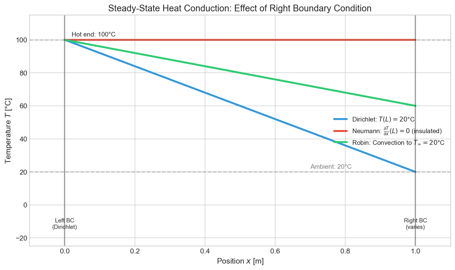
Visualizing the Difference
Consider the 1D heat equation on a rod $[0, L]$ with fixed temperature at $x=0$ and different BCs at $x=L$:
Advanced Boundary Conditions
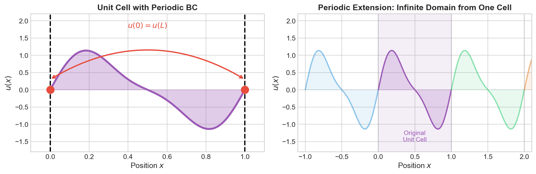
Periodic BC (PBC)
$$u(0, t) = u(L, t), \\ \frac{\partial u}{\partial x}(0, t) = \frac{\partial u}{\partial x}(L, t)$$
Use case: Simulating infinite periodic structures (crystals, waveguides) using a single unit cell.
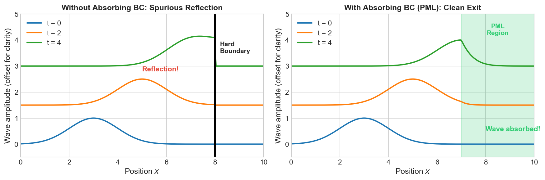
Absorbing BC / Perfectly Matched Layer (PML)
Problem: In wave simulations, boundaries can cause spurious reflections.
Solution: Absorbing BCs or PML layers that “absorb” outgoing waves without reflection.
$$\frac{\partial u}{\partial t} + c\frac{\partial u}{\partial n} = 0 \quad \text{(1st-order absorbing BC)}$$
Use case: Acoustics, electromagnetics, seismic simulations—anywhere you need to model an “infinite” domain.
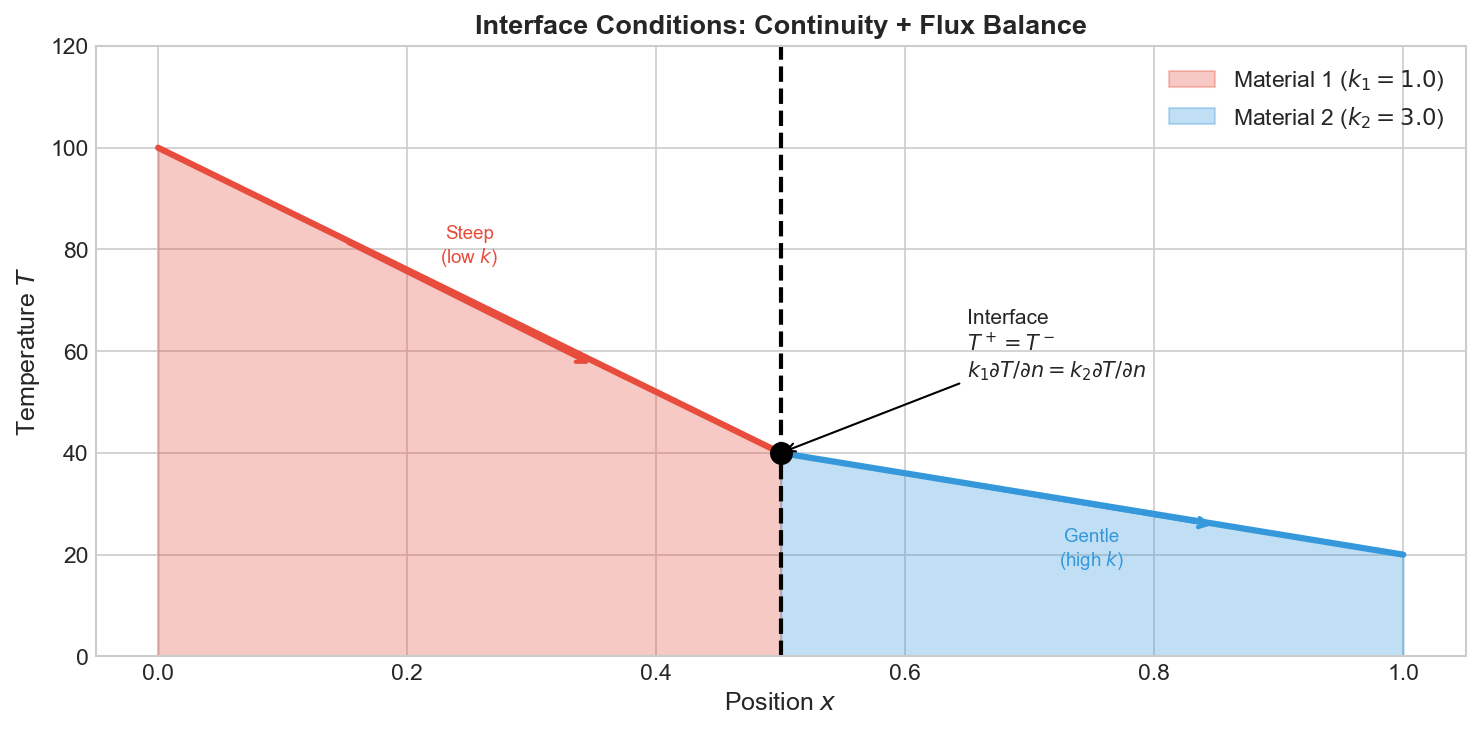
Interface Conditions (IC)
At the interface between two materials:
$$u^+ = u^- \quad \text{(continuity)}$$ $$k^+ \frac{\partial u}{\partial n}^+ = k^- \frac{\partial u}{\partial n}^- \quad \text{(flux balance)}$$
Use case: Composite materials, layered structures, multi-physics problems.
Nonlinear and Time-Varying BCs
In practice, BCs are not always constant:
- Nonlinear BC: Radiative heat transfer follows $q = \sigma \epsilon (T^4 - T_{\infty}^4)$, which is highly nonlinear.
- Time-varying BC: A heating element that cycles on and off: $T(0, t) = f(t)$.
These require iterative solvers and careful time-stepping, but the classification (Dirichlet/Neumann/Robin) still applies.
Matching BCs with PDE Types
Different equation types have different requirements for well-posedness:
| PDE Type | Required Information | Typical BCs |
|---|---|---|
| Elliptic (Laplace) | Value OR flux on entire boundary | Dirichlet, Neumann, or mixed |
| Parabolic (Heat) | Initial condition + BCs on boundary | Dirichlet/Neumann + IC |
| Hyperbolic (Wave) | Initial $u$ and $\partial u/\partial t$ + BCs at inflow | Characteristic BCs |
Common Mistakes
Underdetermined Problem
Mistake: Not specifying enough boundary conditions.
Example: Laplace equation on a square with Neumann BC on all four sides.
Problem: If only flux is given everywhere, the solution is only determined up to a constant. You need at least one Dirichlet condition to “anchor” the solution.
Overdetermined Problem
Mistake: Specifying too many boundary conditions.
Example: Dirichlet on all boundaries PLUS Neumann on all boundaries.
Problem: The problem has no solution unless the BCs happen to be perfectly compatible.
Incompatible BCs
Mistake: BCs that contradict the physics.
Example: Specifying inflow velocity at BOTH ends of a pipe for incompressible flow.
Problem: Mass can’t be conserved.
Summary
| BC Type | Specifies | Physical Example | Mathematical Form |
|---|---|---|---|
| Dirichlet | Value | Fixed temperature | $u = g$ |
| Neumann | Flux | Insulated wall | $\dfrac{\partial u}{\partial n} = h$ |
| Robin | Mixed | Convective cooling | $\alpha u + \beta \dfrac{\partial u}{\partial n} = g$ |
| Periodic | Continuity | Unit cell | $u(0) = u(L)$ |
| Absorbing | Wave exit | Open boundary | $\dfrac{\partial u}{\partial t} + c\dfrac{\partial u}{\partial n} = 0$ |
References
- Evans, L. C. (2010). Partial Differential Equations (2nd ed.). American Mathematical Society.
- Reddy, J. N. (2006). An Introduction to the Finite Element Method (3rd ed.). McGraw-Hill.
- Trefethen, L. N. (2000). Spectral Methods in MATLAB. SIAM.