1D Acoustic Wave Simulation in Heterogeneous Media
Introduction
Acoustic wave simulation is fundamental to many applications, from medical ultrasound imaging to non-destructive testing. Understanding how pressure waves propagate, reflect, and transmit through layered media is essential for designing transducers, interpreting imaging data, and validating theoretical models.
This post explores 1D acoustic wave propagation in a heterogeneous medium—a classic problem that demonstrates key phenomena such as impedance mismatch, partial reflection, and wave speed variation. The simulation is implemented using two complementary tools:
- k-Wave: An open-source MATLAB toolbox using the k-space pseudospectral method
- COMSOL Multiphysics: A commercial finite element software suite
Theoretical Background
The Acoustic Wave Equation
The propagation of acoustic waves in a fluid medium is governed by the linearized equations of fluid mechanics. For a compressible, inviscid fluid, these can be written as coupled first-order partial differential equations:
$$\frac{\partial p}{\partial t} = -\rho_0 c_0^2 \nabla \cdot \mathbf{u}$$
$$\frac{\partial \mathbf{u}}{\partial t} = -\frac{1}{\rho_0} \nabla p$$
where:
- $p$ is the acoustic pressure [Pa]
- $\mathbf{u}$ is the particle velocity [m/s]
- $\rho_0$ is the ambient density [kg/m³]
- $c_0$ is the sound speed [m/s]
In one dimension, these simplify to:
$$\frac{\partial p}{\partial t} = -\rho_0 c_0^2 \frac{\partial u}{\partial x}$$
$$\frac{\partial u}{\partial t} = -\frac{1}{\rho_0} \frac{\partial p}{\partial x}$$
Initial Value Problem (IVP)
An Initial Value Problem specifies the state of the system at $t = 0$ and calculates its evolution over time. In acoustics, this corresponds to scenarios like photoacoustic imaging, where an initial pressure distribution $p_0(x)$ is generated instantaneously (e.g., by laser absorption) and then propagates through the medium.
The initial conditions are: $$p(x, t=0) = p_0(x)$$ $$u(x, t=0) = 0$$
Heterogeneous Medium
In a heterogeneous medium, the material properties $c_0(x)$ and $\rho_0(x)$ vary spatially. This creates:
- Reflection at interfaces due to acoustic impedance mismatch ($Z = \rho_0 c_0$)
- Transmission of the remaining wave energy through the interface
- Speed variation as waves travel faster or slower depending on local properties
The reflection coefficient at a normal interface between two media is:
$$R = \frac{Z_2 - Z_1}{Z_2 + Z_1} = \frac{\rho_2 c_2 - \rho_1 c_1}{\rho_2 c_2 + \rho_1 c_1}$$
Problem Setup
The simulation uses a 1D domain with the following configuration:
| Parameter | Value |
|---|---|
| Domain length | 25.6 mm |
| Grid points | 512 |
| Grid spacing | 0.05 mm |
| Simulation time | ~32 μs |
Heterogeneous Medium Properties
The medium consists of three regions with different acoustic properties:
| Region | Position | Sound Speed | Density | Impedance |
|---|---|---|---|---|
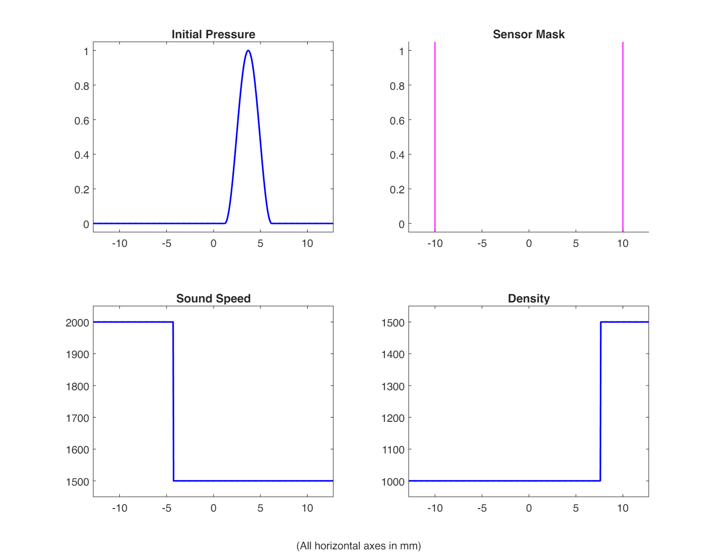
| 1 (left) | x < -4.3 mm | 2000 m/s | 1000 kg/m³ | 2.0 MRayl |
| 2 (middle) | -4.3 mm ≤ x < 7.7 mm | 1500 m/s | 1000 kg/m³ | 1.5 MRayl |
| 3 (right) | x ≥ 7.7 mm | 1500 m/s | 1500 kg/m³ | 2.25 MRayl |
Initial Pressure Distribution
A smooth sinusoidal pulse is placed in region 2, starting at x ≈ 1.2 mm with a width of 5 mm (centered at x ≈ 3.6 mm):
$$p_0(x) = \frac{1}{2}\left[\sin\left(\frac{2\pi(x - x_{start})}{w} - \frac{\pi}{2}\right) + 1\right]$$
for $x_{start} \leq x \leq x_{start} + w$, and $p_0 = 0$ elsewhere.
Sensor Locations
Two sensors are placed symmetrically about the domain center:
- Sensor 1: x = -10 mm
- Sensor 2: x = +10 mm
k-Wave Implementation
k-Wave is an open-source MATLAB toolbox for time-domain acoustic and ultrasound simulations. It uses a k-space pseudospectral method that is highly efficient for wave propagation problems.
Simulation Setup
The k-Wave simulation requires defining four main structures:
| |
Simulation Layout
The following figure shows the simulation setup: initial pressure, sensor locations, sound speed profile, and density profile:
Running the Simulation
Wave Propagation Animation
The following animation shows the acoustic wave propagating through the heterogeneous medium. Notice the reflections at the interfaces and the different propagation speeds in each region:
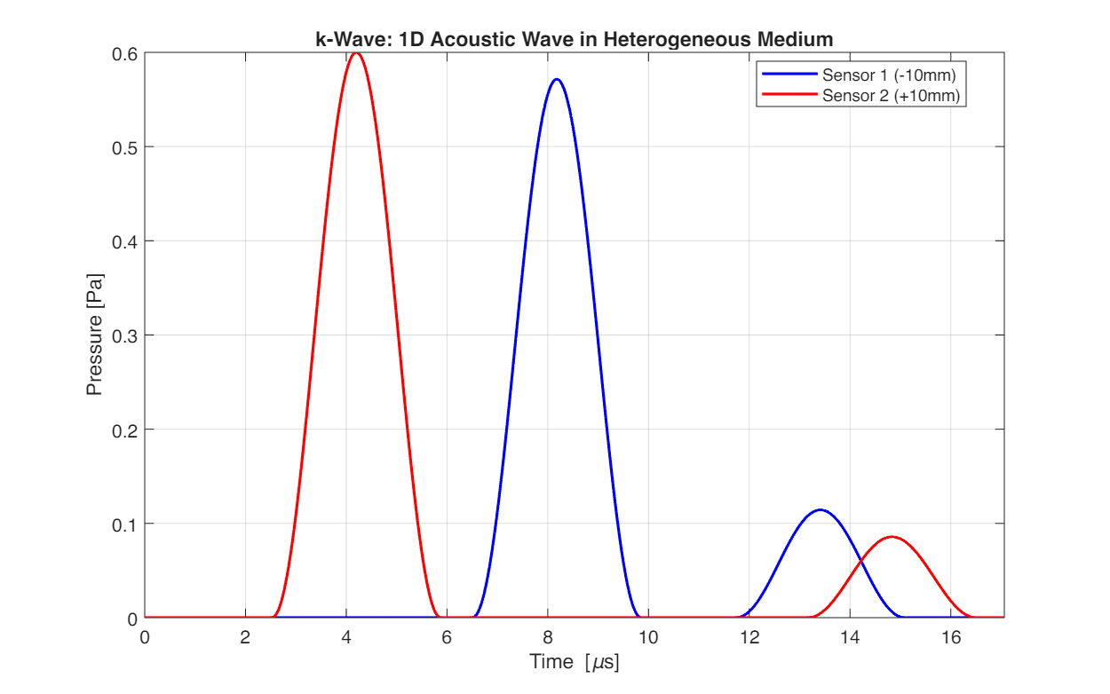
Key observations:
- The initial pulse splits into left-going and right-going waves
- At x ≈ -4.3 mm (interface 1), partial reflection occurs due to impedance mismatch
- At x ≈ 7.7 mm (interface 2), another reflection occurs
- The wave travels faster in region 1 (c = 2000 m/s) than in regions 2 and 3 (c = 1500 m/s)
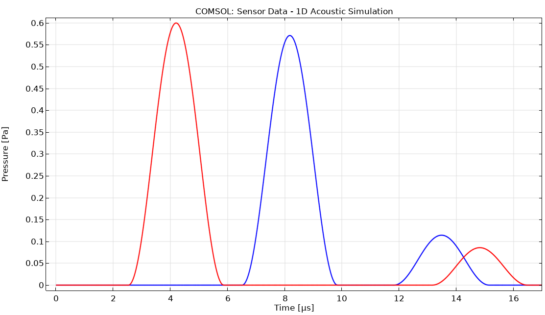
Sensor Results
The pressure recorded at the two sensor positions over time:
COMSOL Implementation
COMSOL Multiphysics uses the Finite Element Method (FEM) to solve the acoustic wave equation. While more computationally expensive, it offers a graphical interface and supports complex geometries.
Model Setup in COMSOL
Create New Model
- Open COMSOL Multiphysics 6.4
- Select Model Wizard → 1D geometry
- Add physics: Acoustics → Pressure Acoustics, Transient
- Select study: Time Dependent
Define Parameters
Go to Global Definitions → Parameters and add:
| Name | Expression | Description |
|---|---|---|
| L_mm | 25.6 [mm] | Domain length |
| c1 | 2000 [m/s] | Sound speed region 1 |
| c2 | 1500 [m/s] | Sound speed regions 2 & 3 |
| rho1 | 1000 [kg/m^3] | Density regions 1 & 2 |
| rho3 | 1500 [kg/m^3] | Density region 3 |
| pulse_width | 5 [mm] | Initial pulse width |
| x_pulse_start | 1.2 [mm] | Pulse start position |
| x_pulse_end | x_pulse_start + pulse_width | Pulse end position |
| p0_amp | 1 [Pa] | Initial pressure amplitude |
| t_end | 32 [μs] | End time |
Build Geometry
- Right-click Geometry 1 → Interval
- Create three intervals corresponding to the three material regions:
- Region 1: [-12.8 mm, -4.3 mm]
- Region 2: [-4.3 mm, 7.7 mm]
- Region 3: [7.7 mm, 12.8 mm]
- Click Build All
Define Materials
Create three materials with properties matching each region:
- Right-click Materials → Blank Material
- For each material, set:
- Sound speed: c1 or c2 as appropriate
- Density: rho1 or rho3 as appropriate
- Assign each material to its corresponding domain
Configure Physics
Initial Values:
- Click on Initial Values 1
- Set Pressure: Enter the initial pulse expression
Boundary Conditions:
- Right-click Pressure Acoustics, Transient → Plane Wave Radiation
- Apply to both end points to simulate absorbing boundaries (equivalent to PML)
Create Mesh
- Right-click Mesh 1 → Edge
- Set Maximum element size to 0.05 mm (matching k-Wave grid)
- Click Build All
Configure Study
- Click Study 1 → Step 1: Time Dependent
- Set Times:
range(0, 0.0125[μs], 32[μs]) - Under Solver Configurations, adjust relative tolerance to 1e-5 for accuracy
Run and Post-Process
- Click Compute
- Create 1D Plot Group for sensor data:
- Add Cut Point 1D datasets at x = -10 mm and x = +10 mm
- Create Point Graph to plot pressure vs. time
COMSOL Results
The COMSOL animation shows the same wave propagation physics:
The COMSOL simulation produces comparable results to k-Wave:
Results Comparison
Sensor Data Overlay
The following figure directly compares the k-Wave and COMSOL results at both sensor positions:
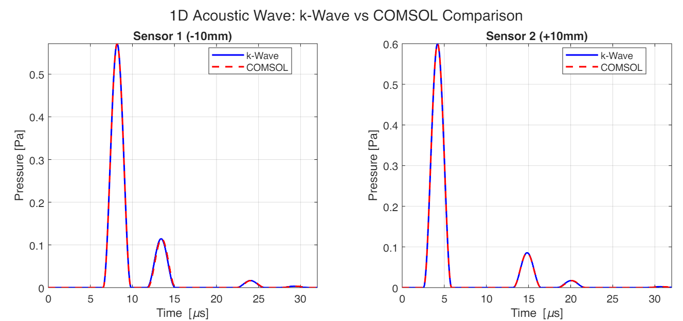
Both simulations show excellent agreement, with the wave arrivals and reflection patterns matching closely.
Efficiency Comparison
One of the most significant differences between k-Wave and COMSOL is computational efficiency.
Benchmark Results
| Parameter | k-Wave | COMSOL |
|---|---|---|
| Grid Points/Elements | 512 | 512 |
| Time Steps | 4267 | 2561 |
| Time Step Size | 0.0075 μs | 0.0125 μs |
| Simulation Time | 0.15 s | 23.31 s |
Speedup Analysis
k-Wave is approximately 155× faster than COMSOL for this 1D acoustic simulation.
This dramatic speedup is due to several factors:
- Algorithm Efficiency: k-Wave uses a k-space pseudospectral method with FFT-based spatial derivatives, which is inherently efficient for wave propagation problems. COMSOL uses FEM, which requires assembling and solving large matrix systems.
- Overhead: COMSOL has significant overhead for model management, GUI updates, and general-purpose infrastructure. k-Wave is purpose-built for acoustic simulations.
- Time Stepping: k-Wave uses an explicit k-space corrected scheme, while COMSOL uses an implicit Generalized-α method. The implicit scheme is more stable but computationally heavier per step.
- Dimensionality: The speedup advantage of k-Wave increases with problem dimensionality (2D, 3D) due to the superior scaling of spectral methods.
When to Use Each Tool
| Scenario | Recommended Tool |
|---|---|
| Large-scale wave propagation (2D/3D) | k-Wave |
| Rapid prototyping and parameter studies | k-Wave |
| Complex geometries (CAD imports) | COMSOL |
| Multi-physics coupling (thermal, structural) | COMSOL |
| Non-acoustic boundary conditions | COMSOL |
| Teaching and visualization | Either |
Conclusion
Both k-Wave and COMSOL successfully simulate 1D acoustic wave propagation in heterogeneous media, producing results that agree well with each other. However, they have different strengths:
- k-Wave excels in computational efficiency, making it ideal for large-scale simulations, parameter sweeps, and inverse problems in medical ultrasound and photoacoustic imaging.
- COMSOL provides greater flexibility for complex geometries, multi-physics coupling, and scenarios where a GUI-based workflow is preferred.
References
- Treeby, B. E., & Cox, B. T. (2010). k-Wave: MATLAB toolbox for the simulation and reconstruction of photoacoustic wave fields. Journal of Biomedical Optics, 15(2), 021314.
- COMSOL Multiphysics Reference Manual, version 6.4.
- Kinsler, L. E., Frey, A. R., Coppens, A. B., & Sanders, J. V. (2000). Fundamentals of Acoustics. John Wiley & Sons.