Introduction

Wave diffraction is one of the most fundamental phenomena in physics, demonstrating how waves bend around obstacles and spread through apertures. When a plane wave encounters a barrier with a slit, the wave diffracts and creates an interference pattern that depends on the ratio of wavelength to slit width.

This post explores 2D acoustic slit diffraction—a classic problem that illustrates Huygens’ principle and wave interference. The simulation is implemented using two complementary tools:

• k-Wave: An open-source MATLAB toolbox using the k-space pseudospectral method
• COMSOL Multiphysics: A commercial finite element software suite

Theoretical Background

Wave Diffraction and Huygens’ Principle

When a plane wave encounters an aperture (slit), each point within the aperture acts as a secondary source of spherical waves (Huygens’ principle). The superposition of these secondary waves produces the diffraction pattern.

For a slit of width $w$ illuminated by a wave of wavelength $\lambda$:

• $\lambda \approx w$: Strong diffraction, nearly hemispherical wave spreading
• $\lambda \ll w$: Weak diffraction, wave passes through with minimal spreading
• $\lambda \gg w$: Very strong diffraction, wave completely spreads

The Acoustic Wave Equation (2D)

In two dimensions, the coupled first-order acoustic equations are:

$$\frac{\partial p}{\partial t} = -\rho_0 c_0^2 \left( \frac{\partial u_x}{\partial x} + \frac{\partial u_y}{\partial y} \right)$$

$$\frac{\partial u_x}{\partial t} = -\frac{1}{\rho_0} \frac{\partial p}{\partial x}$$

$$\frac{\partial u_y}{\partial t} = -\frac{1}{\rho_0} \frac{\partial p}{\partial y}$$

where:

• $p$ is the acoustic pressure [Pa]
• $u_x$, $u_y$ are the particle velocity components [m/s]
• $\rho_0$ is the ambient density [kg/m³]
• $c_0$ is the sound speed [m/s]

High-Impedance Barrier

The barrier is modeled as a region with significantly higher acoustic impedance than the background medium. With an impedance ratio of 20:1, approximately 82% of the incident energy is reflected at the barrier surface (using the intensity reflection coefficient $R = \left(\dfrac{Z_2 - Z_1}{Z_2 + Z_1}\right)^2 \approx 0.82$). This high reflection ensures that most wave energy is blocked, while the remaining portion transmits or diffracts through the slit opening.

Problem Setup

The simulation uses a 2D square domain with the following configuration:

Barrier and Slit Geometry

Source Configuration

A plane wave source is placed at the left boundary, propagating from left to right toward the barrier:

• Source type: Sinusoidal velocity source (plane wave)
• Wavelength: Equal to slit width (3.91 mm)
• Frequency: 384 kHz

When $\lambda \approx w$, significant diffraction occurs, producing a characteristic spreading pattern beyond the slit.

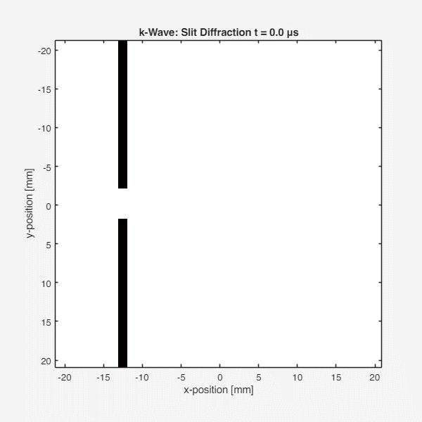
k-Wave Implementation

k-Wave is an open-source MATLAB toolbox for time-domain acoustic and ultrasound simulations. It uses a k-space pseudospectral method that is highly efficient for wave propagation problems.

Simulation Setup

 1
 2
 3
 4
 5
 6
 7
 8
 9
10
11
12
13
14
15
16
17
18
19
20
21
22
23
24
25
26
27
28

% Create computational grid
scale = 1;
Nx = scale * 128;
Ny = Nx;
dx = 50e-3 / Nx;    % grid spacing [m]
dy = dx;
kgrid = kWaveGrid(Nx, dx, Ny, dy);

% Define medium properties
c0 = 1500;          % sound speed [m/s]
rho0 = 1000;        % density [kg/m³]
barrier_scale = 20; % impedance ratio

% Create barrier mask
slit_thickness = scale * 2;     % grid points
slit_width = scale * 10;        % grid points
slit_x_pos = Nx/4;              % left side

slit_offset = Ny/2 - slit_width/2 - 1;
slit_mask = zeros(Nx, Ny);
slit_mask(slit_x_pos:slit_x_pos + slit_thickness, 1:1 + slit_offset) = 1;
slit_mask(slit_x_pos:slit_x_pos + slit_thickness, end - slit_offset:end) = 1;

% Assign barrier properties (high impedance)
medium.sound_speed = c0 * ones(Nx, Ny);
medium.density = rho0 * ones(Nx, Ny);
medium.sound_speed(slit_mask == 1) = barrier_scale * c0;
medium.density(slit_mask == 1) = barrier_scale * rho0;

Source Definition

1
2
3
4
5
6
7
8
9

% Create plane wave source at left boundary
source.u_mask = zeros(Nx, Ny);
source.u_mask(1 + pml_size, :) = 1;

% Sinusoidal source with wavelength = slit width
source_wavelength = slit_width * dx;
source_freq = c0 / source_wavelength;
source_mag = 2 / (c0 * rho0);
source.ux = source_mag * sin(2 * pi * source_freq * kgrid.t_array);

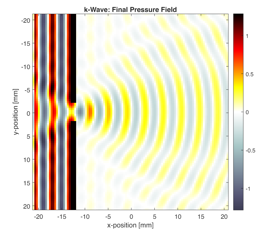
k-Wave Results

The following figure shows the final pressure field after the wave has propagated through the slit:

The wave propagation animation:

Key observations:

1. The plane wave approaches the barrier from the left
2. Most of the wave is blocked by the barrier (high impedance reflection)
3. The wave passes through the slit and diffracts, creating a spreading pattern
4. Interference fringes are visible in the diffracted wave

COMSOL Implementation

COMSOL Multiphysics uses the Finite Element Method (FEM) to solve the acoustic wave equation. The model setup follows similar physical parameters to the k-Wave simulation.

Model Setup

Create New Model

1. Open COMSOL Multiphysics
2. Select Model Wizard → 2D geometry
3. Add physics: Acoustics → Pressure Acoustics, Transient
4. Select study: Time Dependent

Define Geometry

The geometry consists of three rectangular domains:

The barrier is positioned at x = Lx/4 with thickness matching k-Wave (2 grid points = 0.78 mm).

Define Materials

Configure Physics

• Source: Pressure boundary condition on left edge: 2*sin(2*pi*f0*t) (amplitude = 2 Pa). This is equivalent to k-Wave’s velocity source source_mag = 2/(c0*rho0), since $p = \rho_0 c_0 u = 2$ Pa.
• Absorbing BC: Plane Wave Radiation on right, top, and bottom boundaries

Why Plane Wave Radiation instead of PML?
In COMSOL, PML (Perfectly Matched Layer) requires adding additional domain layers around the geometry, which increases model complexity and mesh size. The Plane Wave Radiation boundary condition is a simpler alternative that uses an analytical impedance matching condition to absorb outgoing waves with minimal reflection. For problems with waves primarily traveling perpendicular to boundaries, Plane Wave Radiation provides good absorption with lower computational cost.

Mesh and Solve

• Mesh: Free triangular mesh with at least 6 elements per wavelength
• Time stepping: Adaptive BDF scheme for computational efficiency

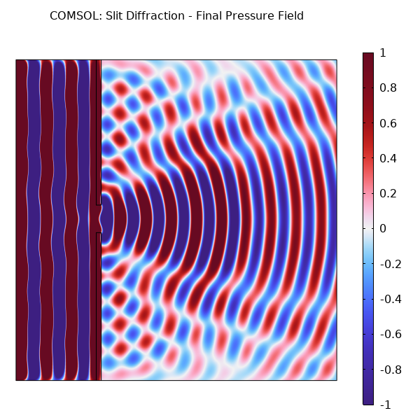
COMSOL Results

The COMSOL simulation produces comparable results to k-Wave:

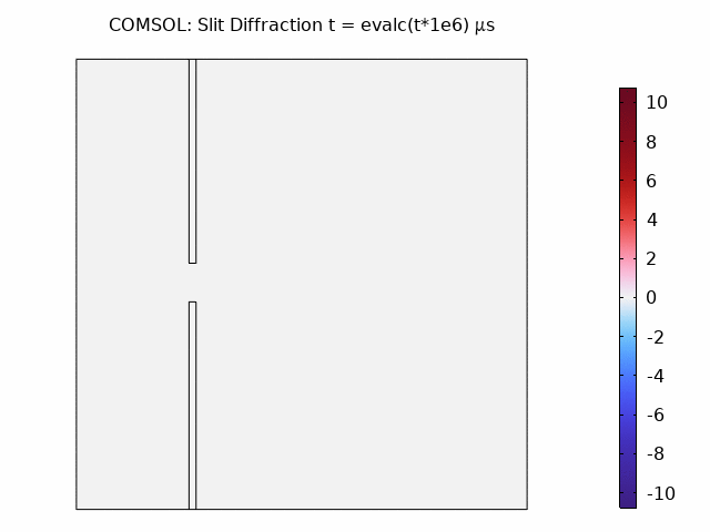
Animation showing wave propagation:

Results Comparison

Visual Comparison

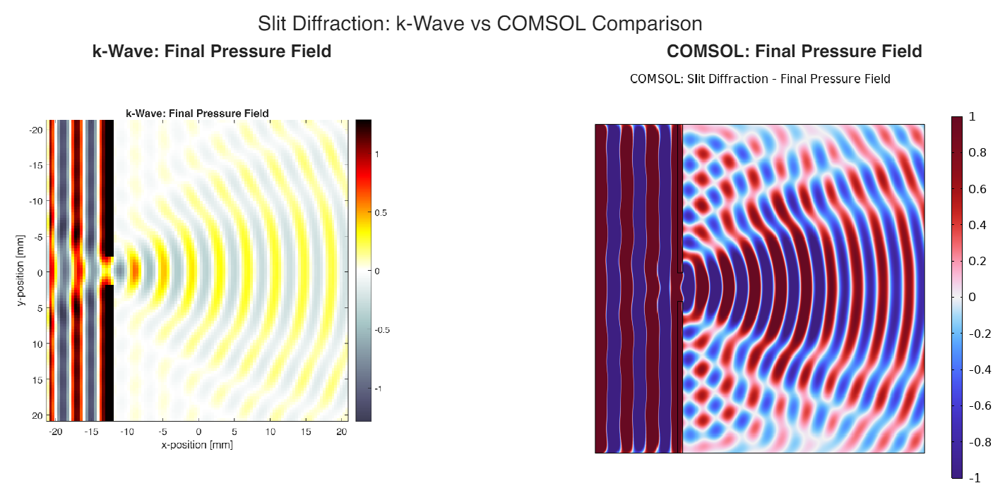
Both simulations show:

• Similar diffraction patterns beyond the slit
• Comparable wave reflection from the barrier
• Matching propagation speed and wavelength

Differences

Some differences are expected due to:

1. Numerical methods: k-Wave uses pseudospectral (FFT-based) spatial derivatives, while COMSOL uses finite elements
2. Boundary conditions: k-Wave uses PML, COMSOL uses Plane Wave Radiation
3. Time stepping: Different schemes (k-space corrected vs. BDF)

Efficiency Comparison

k-Wave is approximately 247× faster than COMSOL for this 2D acoustic slit diffraction simulation.

Conclusion

Both k-Wave and COMSOL successfully simulate 2D acoustic slit diffraction, demonstrating the fundamental wave physics of diffraction and interference. Key findings:

• Wave diffraction through the slit creates a characteristic spreading pattern when $\lambda \approx w$
• k-Wave is highly efficient for wave propagation, ideal for large-scale simulations
• COMSOL provides flexibility and multi-physics capabilities

This simulation demonstrates a classic physics problem that is relevant to:

• Ultrasound imaging
• Non-destructive testing
• Acoustic metamaterials
• Underwater acoustics

References

1. Treeby, B. E., & Cox, B. T. (2010). k-Wave: MATLAB toolbox for the simulation and reconstruction of photoacoustic wave fields. Journal of Biomedical Optics, 15(2), 021314.
2. COMSOL Multiphysics Reference Manual.
3. Hecht, E. (2017). Optics (5th ed.). Pearson. [Diffraction theory applies to all waves]
4. Kinsler, L. E., et al. (2000). Fundamentals of Acoustics. John Wiley & Sons.