ML-07: Nonlinear Regression and Regularization
Learning Objectives
- Transform features for nonlinear regression
- Understand why regularization works
- Implement Ridge regression (L2)
- Choose the regularization strength
Theory
Polynomial Features
Linear regression can only capture straight lines. To model curves, polynomial features transform the input:
$$x \rightarrow (1, x, x^2, x^3, \ldots, x^d)$$
The model becomes:
$$\hat{y} = w_0 + w_1 x + w_2 x^2 + w_3 x^3 + \cdots + w_d x^d$$
Key insight: Despite the curved output, the model remains linear in the parameters $w$. The same normal equation applies—only the feature matrix changes.
| Original Feature | Polynomial Features (degree 3) |
|---|---|
| $x = 2$ | $(1, 2, 4, 8)$ |
| $x = 3$ | $(1, 3, 9, 27)$ |
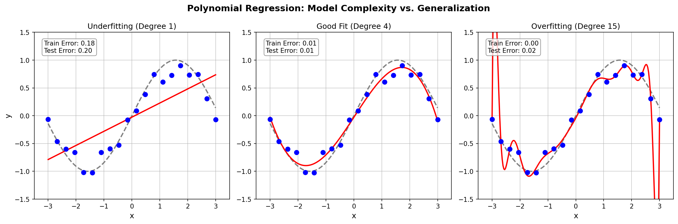
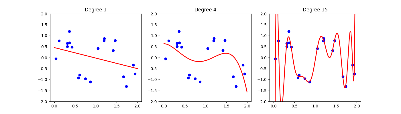
The Overfitting Problem
Higher-degree polynomials have more flexibility to fit training data, but this comes at a cost:
| Degree | Behavior | Training Error | Test Error |
|---|---|---|---|
| Too low (1) | Underfitting — cannot capture the pattern | High | High |
| Just right (4) | Good fit — captures trend without noise | Low | Low |
| Too high (15) | Overfitting — memorizes noise | Very low | Very high |
The Bias-Variance Tradeoff:
- Bias = error from overly simple assumptions (underfitting)
- Variance = error from sensitivity to training data fluctuations (overfitting)
- The optimal model is complex enough to capture the signal, yet simple enough to avoid fitting noise.
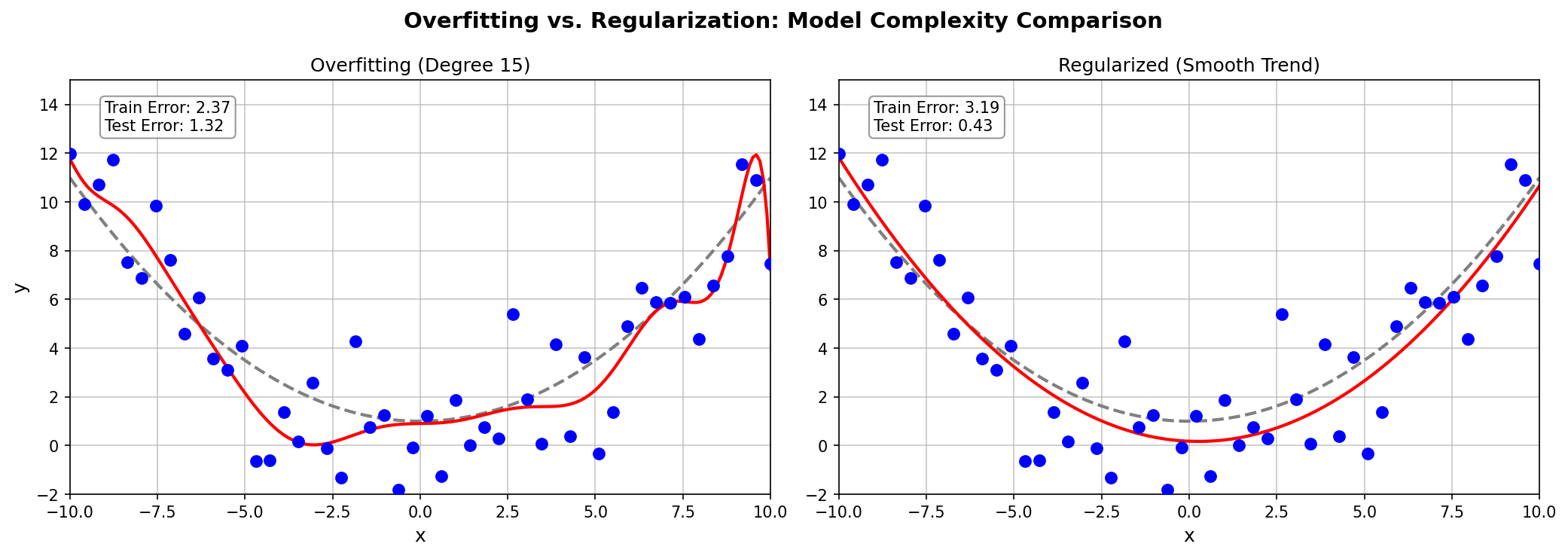
Ridge Regression (L2 Regularization)
Instead of restricting model complexity by limiting degree, regularization adds a penalty term to the loss function:
$$J(\boldsymbol{w}) = |y - Xw|^2 + \lambda |w|^2$$
The first term measures data fit (prediction error), while the second term is the penalty (weight magnitude).
Why does penalizing large weights help?
- Large weights enable sharp oscillations in the fitted curve
- Constraining weights to remain small produces smoother curves
- Smaller weights correspond to simpler, more generalizable models
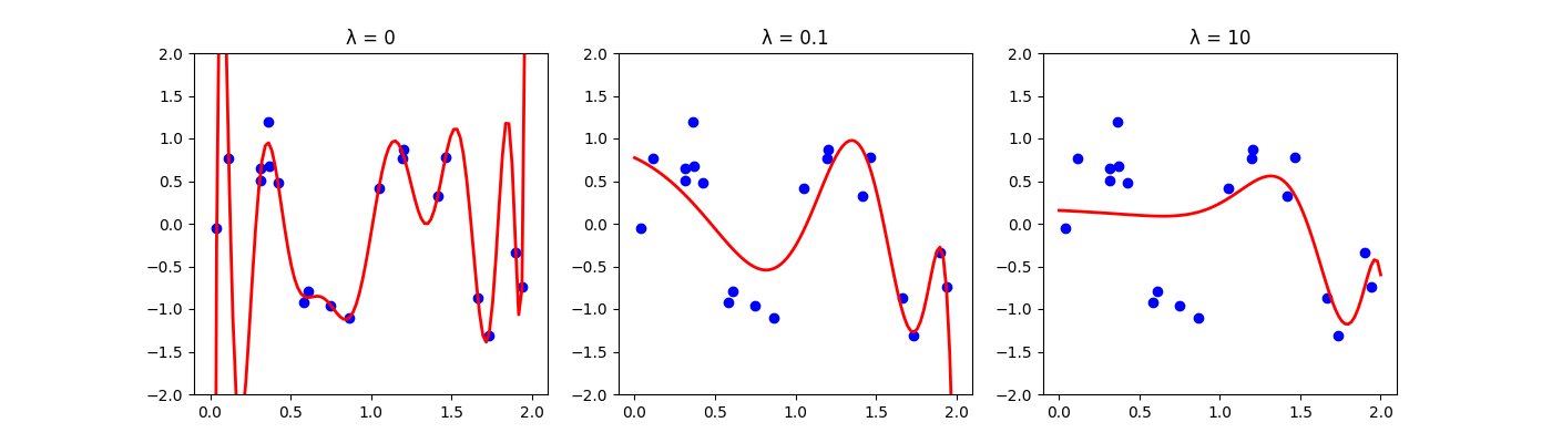
| $\lambda$ | Effect | Resulting Model |
|---|---|---|
| 0 | No regularization = ordinary least squares | May overfit |
| Small | Light constraint on weights | Slight smoothing |
| Large | Heavy constraint → weights shrink toward 0 | May underfit |
Closed-Form Solution
The Ridge regression solution has a closed form:
$$\boldsymbol{w}^* = (X^T X + \lambda I)^{-1} X^T y$$
Comparing to standard linear regression:
| Method | Solution | Matrix Invertibility |
|---|---|---|
| OLS | $(X^T X)^{-1} X^T y$ | Can fail if $X^T X$ is singular |
| Ridge | $(X^T X + \lambda I)^{-1} X^T y$ | Always invertible (λI ensures positive definiteness) |
💡 Tip: Ridge regression solves two problems at once: it prevents overfitting AND guarantees a solution even when features are collinear.
Code Practice
Polynomial Overfitting Demo
🐍 Python
| |
Ridge Regression Comparison
🐍 Python
| |
Finding Optimal λ with Cross-Validation
🐍 Python
| |
Output:
| |
Deep Dive
FAQ
Q1: Ridge vs. Lasso — what’s the difference?
| Regularization | Penalty | Effect on Weights | Best For |
|---|---|---|---|
| Ridge (L2) | $\lambda |w|^2$ | Shrinks all weights toward zero | When all features contribute |
| Lasso (L1) | $\lambda |w|_1$ | Can set weights exactly to zero | Feature selection |
| Elastic Net | Both L1 + L2 | Combines benefits of both | Many correlated features |
Geometric intuition:
- Ridge penalty creates a circular constraint region → weights shrink but never reach exactly zero
- Lasso penalty creates a diamond-shaped region → solutions tend to land on corners (sparse weights)
Q2: How do I choose between polynomial degrees?
Use cross-validation with the “one standard error rule”:
- Try degrees 1 through 10 (or higher)
- Compute cross-validation score for each degree
- Find the degree with the best average score
- Select the simplest model (lowest degree) within 1 standard error of the best
Q3: Why is sklearn’s parameter called alpha instead of λ?
This is purely a naming convention. In sklearn:
alpha= $\lambda$ (regularization strength)- Higher alpha = more regularization = smaller weights = smoother curves
Q4: When should I use polynomial regression vs. other nonlinear methods?
| Method | Pros | Cons |
|---|---|---|
| Polynomial Regression | Simple, interpretable, fast | Can overfit, limited patterns |
| Splines | Smooth, local flexibility | Harder to interpret |
| Decision Trees | Captures complex patterns | Prone to overfitting |
| Neural Networks | Universal approximators | Need lots of data, black box |
Summary
| Concept | Key Points |
|---|---|
| Polynomial Features | Enable nonlinear fitting with linear model |
| L2 Regularization | $\lambda |w|^2$ penalty shrinks weights |
| Ridge Solution | $(X^T X + \lambda I)^{-1} X^T y$ |
| λ Selection | Use cross-validation |
References
- Hastie, T. et al. “The Elements of Statistical Learning” - Chapter 3
- sklearn Ridge Regression
- Hoerl, A. & Kennard, R. (1970). “Ridge Regression”