Master GMM: The 'Explorer in the Fog' of clustering. Learn how to map overlapping 'hills' of data, handle uncertainty with soft clustering, and master the EM algorithm.
Learning Objectives
After reading this post, you will be able to:
Understand Gaussian Mixture Models as a probabilistic clustering approach
Know the difference between hard and soft clustering
Understand the Expectation-Maximization (EM) algorithm
Choose between GMM and K-Means for your clustering tasks
Theory
The Intuition: The Explorer in the Fog
K-Means (Clear Day): You are mapping islands in bright sunlight. The boundaries are sharp. You are either on Island A or Island B.
GMM (Foggy Terrain): You are mapping hills in a thick fog. You can’t see the edges clearly. You stand at a point and say: “I am 70% sure I’m on Hill A, but there’s a 30% chance I’m actually on the lower slope of Hill B.”
Gaussian Mixture Models (GMM) embrace this uncertainty using soft clustering.
$\mathcal{N}(x | \mu, \Sigma)$ = Gaussian probability density
Think of it as a recipe:
A GMM is like a smoothie made of $K$ different fruits.
The Fruit ($\mathcal{N}$): The base flavor (the shape of the distribution).
The Amount ($\pi_k$): How much of each fruit you put in (e.g., 70% Strawberry, 30% Banana).
The Result ($p(x)$): The final mixture that describes your entire dataset.
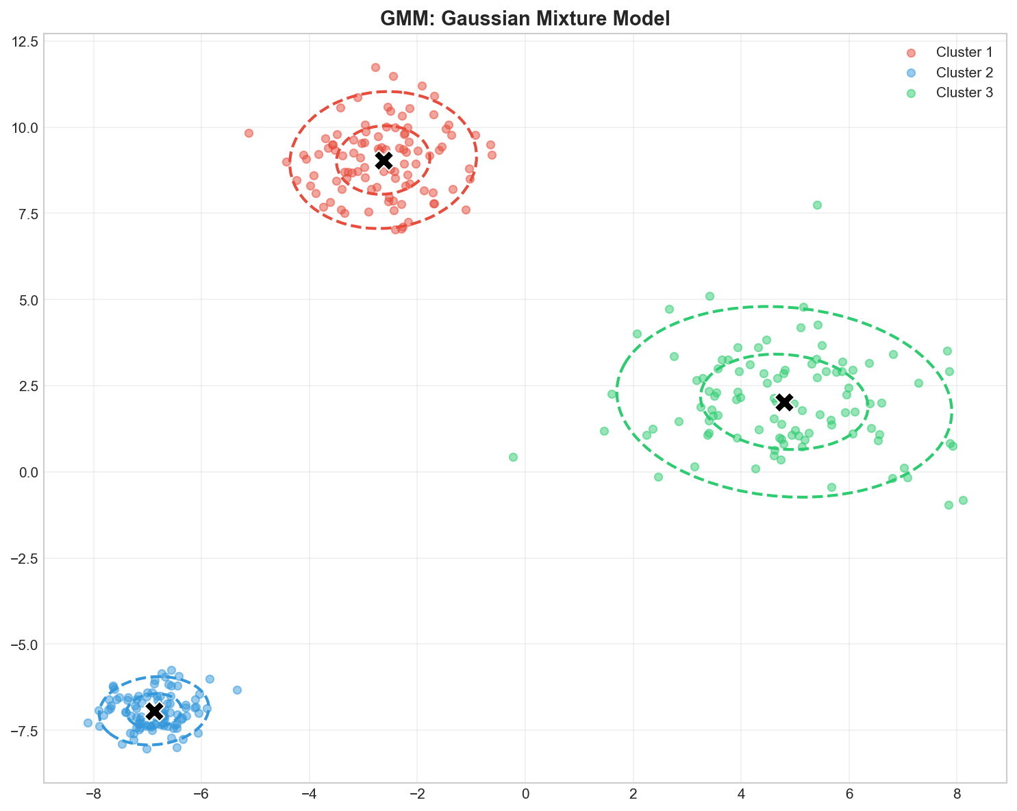
GMM: Each cluster is a Gaussian distribution with its own mean, covariance, and weight
GMM vs K-Means
Aspect
K-Means
GMM
Assignment
Hard (0 or 1)
Soft (probabilities)
Cluster shape
Spherical only
Elliptical (any covariance)
Model
Distance-based
Probabilistic
Parameters
Centroids only
Mean, covariance, weights
Output
Cluster labels
Probabilities + labels
The EM Algorithm
GMM parameters are learned using the Expectation-Maximization (EM) algorithm:
graph LR
subgraph Loop ["The Surveyor's Loop (EM Algorithm)"]
direction LR
A["Guess Initial Locations"] --> B["E-Step: Estimate Membership\n(Where are the points?)"]
B --> C["M-Step: Update Map\n(Move peaks to center of mass)"]
C --> D{"Map Stabilized?"}
D -->|No| B
D -->|Yes| E["Final Map Created"]
end
style B fill:#e1f5fe
style C fill:#fff9c4
style E fill:#c8e6c9
E-Step: The “Where am I?” Phase
We look at every point and ask: “Given our current map of the hills, how likely is it that you belong to Hill A vs Hill B?”
We calculate the Responsibility ($\gamma_{ik}$): The probability that point $i$ implies cluster $k$.
If a point is right in the middle of Hill A’s peak, it gets a high probability for A (e.g., 0.99).
If it’s in the foggy valley between A and B, it might get split (0.5 for A, 0.5 for B).
Now that we have a better idea of who belongs where, we update the map boundaries to fit the data better.
Update Weights ($\pi_k$): Did Hill A get more points assigned to it? Make Hill A “bigger” (increase weight).
Update Means ($\mu_k$): Calculate the weighted average of all points assigned to Hill A. Move the peak to this new center.
Update Covariances ($\Sigma_k$): Did the points spread out? Widen the hill. Did they bunch up? Narrow the hill.
The Cycle: We repeat this “Guess -> Check -> Update” loop until the map stops changing (Convergence). This guarantees we find a local optimum!
Covariance: The Shape of the Hill
Each cluster (hill) can have a different shape. The covariance_type parameter defines what these hills can look like:
Type
Analogy
Shape Flexibility
Parameters
spherical
Perfect Dome
Round only. Width is same in all directions.
Lowest (Simple)
diag
Oval Dome
Stretched along axes (North-South or East-West), but not tilted.
Medium
full
Any Hill
Any shape, any tilt. Can be long, thin, and diagonal.
Highest (Complex)
tied
Clone Hills
All hills must have the exact same shape and size.
High
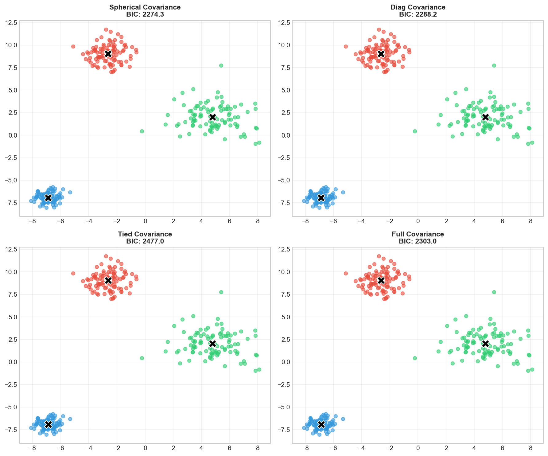
Different covariance types: spherical (circles), diagonal (axis-aligned ellipses), full (any ellipse)
Model Selection: Choosing K
Unlike K-Means, GMM provides principled ways to choose $K$:
1. AIC (Akaike Information Criterion)
$$AIC = 2k - 2\ln(\hat{L})$$
2. BIC (Bayesian Information Criterion)
$$BIC = k\ln(N) - 2\ln(\hat{L})$$
where $k$ = number of parameters, $\hat{L}$ = maximum likelihood.
Occam’s Razor: BIC penalizes complexity ($k \ln N$) more strongly than AIC ($2k$). Use BIC if you want a simpler model with fewer clusters. Use AIC if you care more about fitting the data perfectly, even if it’s complex.
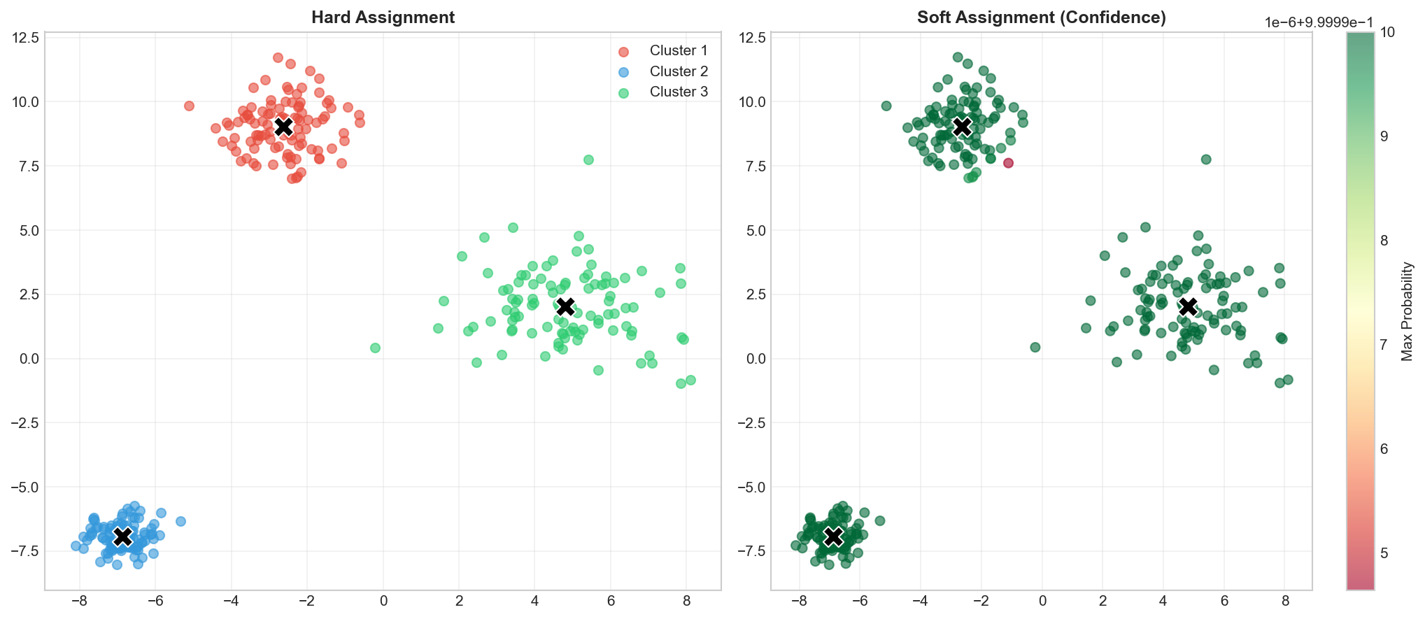
# Visualize soft assignmentsfig,axes=plt.subplots(1,2,figsize=(14,6))colors=['#e74c3c','#3498db','#2ecc71']# Hard clusteringforkinrange(3):mask=labels==kaxes[0].scatter(X[mask,0],X[mask,1],c=colors[k],alpha=0.6,s=40,label=f'Cluster {k+1}')axes[0].scatter(gmm.means_[:,0],gmm.means_[:,1],c='black',marker='X',s=200,edgecolors='white')axes[0].set_title('Hard Assignment (predict)',fontsize=12,fontweight='bold')axes[0].legend()axes[0].grid(True,alpha=0.3)# Soft clustering - color by max probabilitymax_prob=probs.max(axis=1)scatter=axes[1].scatter(X[:,0],X[:,1],c=max_prob,cmap='RdYlGn',alpha=0.6,s=40)axes[1].scatter(gmm.means_[:,0],gmm.means_[:,1],c='black',marker='X',s=200,edgecolors='white')plt.colorbar(scatter,ax=axes[1],label='Max Probability')axes[1].set_title('Soft Assignment (probability)',fontsize=12,fontweight='bold')axes[1].grid(True,alpha=0.3)plt.tight_layout()plt.savefig('assets/gmm_soft_clustering.png',dpi=150)plt.show()
Left: Hard assignments. Right: Colored by confidence — uncertain points (yellow) are near cluster boundaries
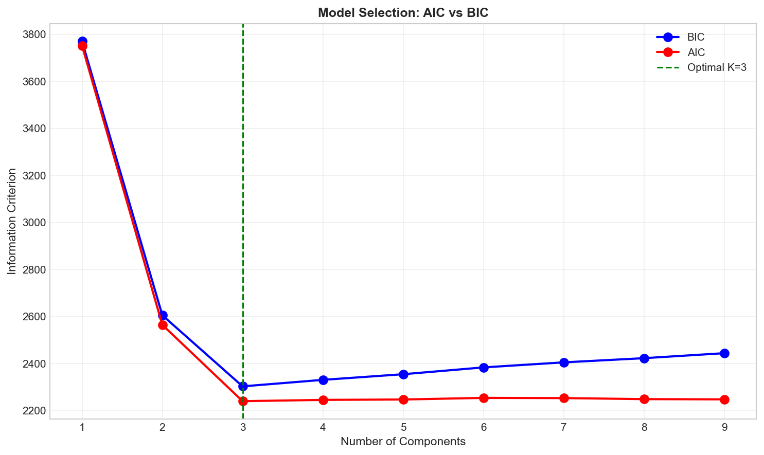
# Find optimal number of componentsn_components_range=range(1,10)bics=[]aics=[]forninn_components_range:gmm=GaussianMixture(n_components=n,random_state=42)gmm.fit(X)bics.append(gmm.bic(X))aics.append(gmm.aic(X))# Plotfig,ax=plt.subplots(figsize=(10,6))ax.plot(n_components_range,bics,'bo-',label='BIC',linewidth=2,markersize=8)ax.plot(n_components_range,aics,'ro-',label='AIC',linewidth=2,markersize=8)ax.axvline(x=3,color='green',linestyle='--',label='Optimal K=3')ax.set_xlabel('Number of Components',fontsize=11)ax.set_ylabel('Information Criterion',fontsize=11)ax.set_title('Model Selection: AIC vs BIC',fontsize=12,fontweight='bold')ax.legend()ax.grid(True,alpha=0.3)plt.tight_layout()plt.savefig('assets/gmm_model_selection.png',dpi=150)plt.show()print(f"\n📊 Optimal K (BIC): {np.argmin(bics)+1}")print(f"📊 Optimal K (AIC): {np.argmin(aics)+1}")
Both AIC and BIC reach minimum at K=3, confirming our true number of clusters
Deep Dive
When to Use GMM vs K-Means
Scenario
Recommendation
Need probability estimates
GMM
Elliptical clusters
GMM (full covariance)
Only spherical clusters
K-Means (faster)
Large datasets
K-Means (more scalable)
Need principled K selection
GMM (use BIC)
Overlapping clusters
GMM
GMM Limitations
Sensitive to initialization — use multiple restarts (n_init)
Can fail with few samples — needs enough data per cluster
Covariance estimation issues — may hit singular matrices
Assumes Gaussian clusters — fails on non-Gaussian shapes
Frequently Asked Questions
Q1: How do I handle singular covariance matrices?
Options:
Add regularization: reg_covar=1e-6
Use simpler covariance: covariance_type='diag'
Get more data per cluster
Q2: Can GMM detect outliers?
Yes! Points with low probability under all components are potential outliers: