Mat Model Lab: An Open-Source Tool for Material Constitutive Model Analysis and Visualization
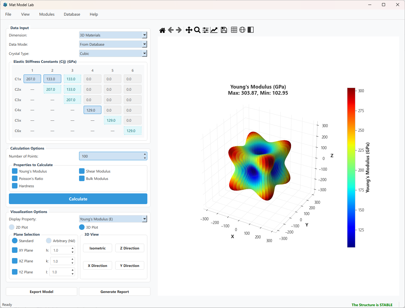
First-principles calculations or experiments hand you a $6 \times 6$ stiffness matrix — and then what? Extracting directional Young’s modulus, checking mechanical stability, computing polycrystalline averages, and exporting material cards for ABAQUS or COMSOL usually means writing one-off scripts every time. Mat Model Lab packages all of that into a single, open-source desktop application so you can go from raw $C_{ij}$ to publication-ready 3D anisotropy plots in seconds.
GitHub: github.com/seekzzh/mat-model-lab
Why Build This Tool?
In computational materials science, the elastic constant matrix ($C_{ij}$) is fundamental to describing the mechanical behavior of materials. First-principles calculations (e.g., VASP, Quantum ESPRESSO) or experimental measurements can provide a $6 \times 6$ stiffness matrix, but there is a significant gap between a raw matrix and engineering intuition:
- How do you intuitively visualize the directional dependence of Young’s modulus in anisotropic materials?
- What are the Voigt, Reuss, and Hill polycrystalline average values?
- Does a given set of elastic constants satisfy the Born stability criteria?
- How do you export elastic parameters as an ABAQUS UMAT or COMSOL material card?
Mat Model Lab was created to bridge this gap.
Core Features
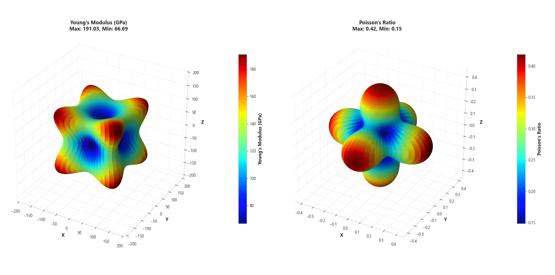
Directional Elastic Property Visualization
Mat Model Lab supports 2D (polar) and 3D (spherical) directional visualization of the following elastic properties:
| Property | Formula Basis | Dimensionality |
|---|---|---|
| Young’s Modulus $E(\theta, \varphi)$ | $E = 1/S’_{11}$ | 3D |
| Shear Modulus $G(\theta, \varphi, \chi)$ | $G = 1/(4S’_{66})$ | 4D → Cross-section |
| Poisson’s Ratio $\nu(\theta, \varphi, \chi)$ | $\nu = -S’{12}/S’{11}$ | 4D → Cross-section |
| Bulk Modulus $B(\theta, \varphi)$ | $B = 1/(S_{11}+S_{12}+S_{13})\dots$ | 3D |
| Hardness $H(\theta, \varphi)$ | Chen-Niu Model | 3D |
All directional properties are computed from the compliance matrix $\mathbf{S} = \mathbf{C}^{-1}$ via rotation transformations. For 4D properties (e.g., shear modulus depends on an additional angle $\chi$), the software averages over $\chi$ on a specified cross-section.
Stiffness vs. Compliance
- The stiffness matrix $\mathbf{C}$ maps strain → stress ($\sigma = \mathbf{C}\varepsilon$).
- The compliance matrix $\mathbf{S} = \mathbf{C}^{-1}$ maps stress → strain. Directional properties like $E(\theta,\varphi)$ are most naturally expressed through $\mathbf{S}$.
Crystal Symmetry Types
A material’s crystal symmetry determines how many independent elastic constants it has — from 21 for Triclinic (no symmetry) down to just 3 for Cubic. Choosing the correct symmetry class is the first step in any elastic analysis, as it dictates which $C_{ij}$ entries are independent, which are related by symmetry, and which are zero.
The software includes built-in definitions for the complete set of 3D crystal symmetry types:
The numbers in parentheses indicate the count of independent elastic constants. After selecting a crystal type, the input panel automatically disables non-independent entries and fills the matrix based on symmetry relations during computation.
Additionally, 2D materials (Hexagonal, Square, Rectangular, Oblique) are supported, suitable for elastic analysis of two-dimensional materials such as graphene and $\text{MoS}_2$.
Voigt-Reuss-Hill Polycrystalline Averaging
For polycrystalline materials, the software automatically computes:
- Voigt upper bound (equal strain assumption)
- Reuss lower bound (equal stress assumption)
- Hill average: $X_{\text{Hill}} = (X_{\text{Voigt}} + X_{\text{Reuss}}) / 2$
Output includes: Bulk modulus $K$, Shear modulus $G$, Young’s modulus $E$, and Poisson’s ratio $\nu$.
A single crystal has direction-dependent properties, but a polycrystal (many randomly oriented grains) behaves isotropically on average. The Voigt bound assumes uniform strain across all grains (upper estimate), Reuss assumes uniform stress (lower estimate), and Hill simply takes the arithmetic mean of the two — a practical and widely cited approximation.
Born Stability Check
After entering elastic constants, the software automatically verifies that all eigenvalues of the stiffness matrix are positive. If the material is mechanically unstable, the interface clearly marks it as “The Structure is UNSTABLE”.
Finite Element Code Export
Elastic constants can be exported with one click to:
- ABAQUS UMAT (Fortran
.ffile) - COMSOL Parameters (
.txtfile)
Report Generation
Analysis reports can be exported in three formats:
| Format | Description |
|---|---|
| HTML | Interactive report, opens in browser |
| Printable document | |
| Word | Editable .docx file |
Reports include: material information, $C_{ij}/S_{ij}$ matrices, VRH results, stability analysis, and visualization charts for all elastic properties.
Technical Architecture
| |
Technology Stack
| Technology | Purpose |
|---|---|
| Python 3.9+ | Core language |
| PyQt6 | GUI framework |
| NumPy / SciPy | Matrix operations and linear algebra |
| Matplotlib | 2D/3D scientific visualization |
| pandas / openpyxl | Excel data I/O |
| python-docx | Word report generation |
Design Highlights
- Separation of computation and GUI: The
core/modules are pure NumPy functions with no GUI dependencies, usable as a standalone Python library. - Modular architecture: Elasticity, Plasticity, and Hyperelasticity are independent modules plugged into the main window.
- Dark/Light theme: One-click toggle with all controls and charts adapting automatically.
- Cross-platform: Built on PyQt6, runs on Windows, macOS, and Linux.
Getting Started
Option A: Download the Executable
Download MatModelLab.exe from the
Releases
page. Double-click to run — no Python installation required.
Option B: Run from Source
Option C: Use as a Python Library
| |
Worked Example: Analyzing Elastic Anisotropy of Copper
- Launch the program → Select Data Mode: “From Database”
- Load material → Database → Browse Materials → Select Copper (Pure)
- Choose visualization → 3D mode, check Young’s Modulus
- Click Calculate
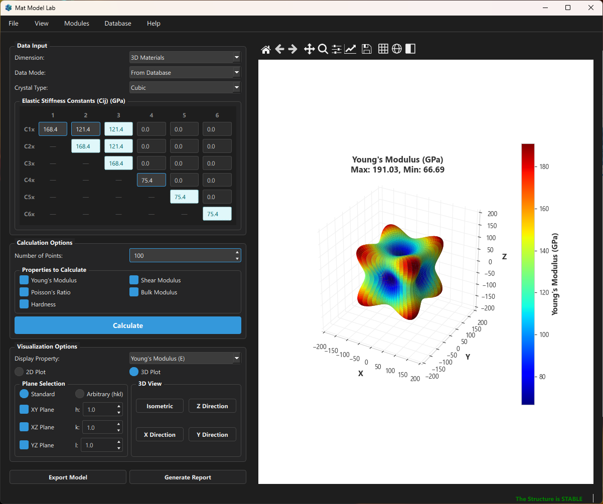
The results show that the anisotropy ratio of Cu is $A = 2C_{44}/(C_{11}-C_{12}) \approx 3.21$, making it a strongly anisotropic FCC metal. The 3D plot clearly shows that Young’s modulus is maximum along the $[111]$ direction and minimum along the $[100]$ direction.
2D Material Support
Mat Model Lab includes dedicated support for elastic analysis of two-dimensional materials. Taking graphene as an example:
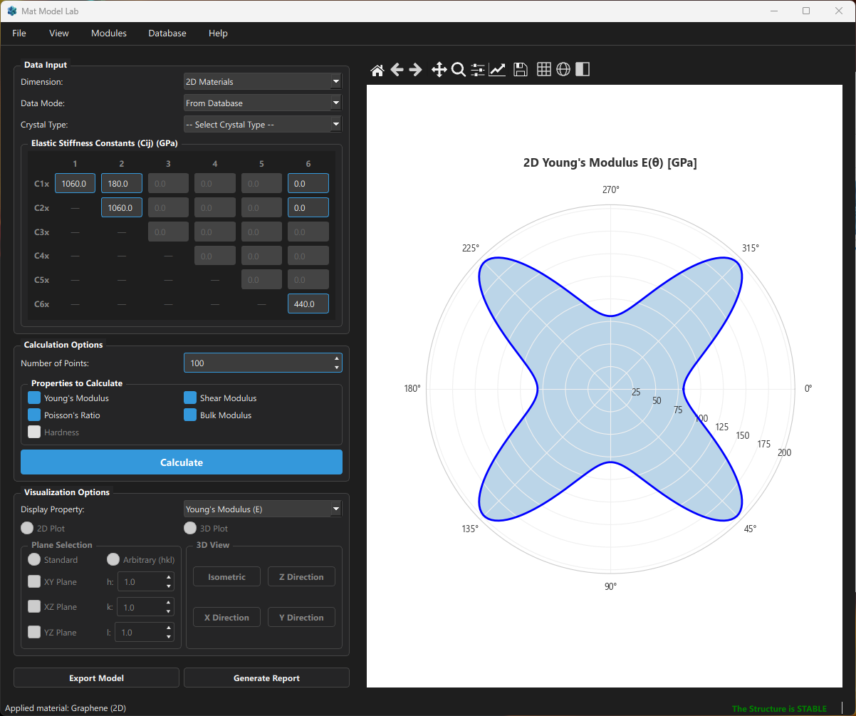
Graphene belongs to the 2D Hexagonal symmetry type, with isotropic in-plane elastic properties — the polar plot forms a perfect circle.
Future Roadmap
- 🚧 Plasticity module: von Mises, Hill, and Drucker-Prager yield criteria with stress-strain curve fitting
- 🚧 Hyperelasticity module: Parameter calibration and UMAT generation for Neo-Hookean, Mooney-Rivlin, Ogden, and other models
- 📋 GitHub Actions CI for automated testing
- 📋 Comprehensive pytest unit test suite
Contributing
Contributions are welcome through:
- 🐛 File a Bug Report
- 💡 Submit a Feature Request
- 🔧 Open a Pull Request
See CONTRIBUTING.md for details.
License: GPL-3.0 | GitHub: seekzzh/mat-model-lab