Necking of an Elastoplastic Metal Bar: COMSOL vs Abaqus Implementation
When a ductile metal bar is stretched beyond its yield point, an interesting phenomenon occurs: instead of deforming uniformly, the bar develops a localized constriction—a “neck”—that eventually leads to fracture. This necking instability is a cornerstone benchmark for validating large-strain elastoplasticity in finite element codes.
In this tutorial, we implement the same necking simulation in two industry-leading FEA platforms: COMSOL Multiphysics and Abaqus/Standard. By comparing their approaches, we gain insights into how different software handles this challenging nonlinear problem.
In this post, we will:
- Understand the Physics: Explore the mechanics behind necking instability.
- Define the Material Model: Implement nonlinear isotropic hardening with combined Voce and linear terms.
- Compare Implementations: Contrast COMSOL MATLAB scripting with Abaqus Python scripting.
- Analyze Results: Visualize necking evolution and interpret force-displacement curves.
The Physics: Why Does Necking Occur?
The Considère Criterion
During uniaxial tension, two competing effects determine stability:
- Strain hardening: The material becomes stronger as plastic strain accumulates.
- Geometric softening: The cross-sectional area decreases as the bar elongates.
The onset of necking occurs when geometric softening overtakes strain hardening. Mathematically, this is captured by the Considère criterion:
$$ \frac{d\sigma}{d\varepsilon} = \sigma $$
Where $\sigma$ is the true stress and $\varepsilon$ is the true strain. When the hardening rate equals the current stress, uniform deformation becomes unstable, and localization begins.
Triggering the Instability
In a perfect cylinder, necking would theoretically occur everywhere simultaneously (an indeterminate problem). To trigger localized necking in simulations, we introduce a small geometric imperfection—a slight reduction in radius at the symmetry plane.
In our models, the imperfection amplitude is:
$$ \Delta R = 0.002 \times R_0 = 0.0128 \text{ mm} $$
This tiny perturbation (0.2% of the radius) is enough to break symmetry and initiate necking at the center.
Material Model: Nonlinear Isotropic Hardening
We model the bar as an elastoplastic steel with combined Voce (exponential saturation) and linear hardening:
$$ \sigma_h(\varepsilon_{pe}) = H \cdot \varepsilon_{pe} + (\sigma_{SF} - \sigma_0) \left(1 - e^{-\zeta \cdot \varepsilon_{pe}}\right) $$
Where:
- $\sigma_0 = 450$ MPa — Initial yield stress
- $\sigma_{SF} = 715$ MPa — Saturation flow stress
- $H = 129.24$ MPa — Linear hardening modulus
- $\zeta = 16.93$ — Saturation exponent
- $\varepsilon_{pe}$ — Equivalent plastic strain
This model captures realistic metal behavior: rapid initial hardening that gradually saturates, combined with a linear term that persists at large strains.
Elastic Properties
| Property | Value |
|---|---|
| Young’s modulus | 206.9 GPa |
| Poisson’s ratio | 0.29 |
| Density | 7850 kg/m³ |
Geometry and Boundary Conditions
We exploit symmetry to model only half the bar (from z = 0 to z = H₀/2):
| Parameter | Value |
|---|---|
| Total bar length | 53.334 mm |
| Bar radius | 6.413 mm |
| Modeled length | 26.667 mm |
| Imperfection | 0.0128 mm |
| Max displacement | 10 mm |
Boundary Conditions
- Symmetry plane (z = 0): Zero normal displacement (uz = 0)
- Top face (z = H₀/2): Prescribed axial displacement (δ = 0 → 10 mm)
- Center point (origin): Fixed in x-y to prevent rigid body motion
Implementation Comparison
Overview: COMSOL vs Abaqus
| Aspect | COMSOL Multiphysics | Abaqus/Standard |
|---|---|---|
| Scripting Language | MATLAB | Python |
| Geometry Creation | Work plane + Revolve | Sketch + BaseSolidRevolve |
| Strain Formulation | Total Lagrangian | NLGEOM=ON (Updated Lagrangian) |
| Strain Decomposition | Additive | Multiplicative (default) |
| Hardening Input | Analytic function | Tabular data (50 points) |
| Element Type | 10-node tetrahedral | C3D10 (10-node tet) |
| Solver | Fully coupled, auto-damping | Newton-Raphson |
| Parametric Loading | Built-in parametric sweep | Single step with increments |
COMSOL Implementation Highlights
In COMSOL, we create the geometry by defining a 2D profile on a work plane and revolving it 360° around the axis. The imperfection is built into the profile: the radius at z = 0 is slightly smaller than at z = H₀/2.
The material hardening is defined as an analytic function directly in the material property group. This allows COMSOL to compute derivatives automatically for the consistent tangent stiffness.
| |
The simulation uses a parametric stationary study that sweeps the displacement parameter from 0 to 10 mm in 41 steps (0.25 mm increments). This provides fine resolution of the necking evolution.
Key physics settings include:
- Total Lagrangian formulation for large strains
- Additive strain decomposition (logarithmic strains)
- Reduced integration to prevent volumetric locking
Abaqus Implementation Highlights
In Abaqus, geometry creation follows a similar revolve approach, but the Python API differs significantly. The sketch is created with explicit point coordinates and then revolved.
Since Abaqus requires tabular hardening data, we generate 50 data points from the hardening function before defining the material. This discretization captures the nonlinear hardening curve accurately.
| |
Key differences in the Abaqus approach:
- NLGEOM=ON activates geometric nonlinearity
- A single Static step with automatic time incrementation
- History output requests track reaction forces and displacements
- C3D10 elements (10-node modified tetrahedra) for accuracy
The boundary condition application uses set-based regions identified by bounding box coordinates, similar to COMSOL’s box selections.
Mesh Configuration
Both implementations use 10-node tetrahedral elements with local refinement near the necking zone (z = 0):
| Mesh Parameter | COMSOL | Abaqus |
|---|---|---|
| Element type | FreeTet (order 2) | C3D10 |
| Global size | R₀/4 ≈ 1.6 mm | R₀/4 ≈ 1.6 mm |
| Refinement zone | Bottom face | Bottom face |
| Refined size | R₀/6 ≈ 1.1 mm | R₀/6 ≈ 1.1 mm |
The mesh refinement at the symmetry plane ensures adequate resolution as the neck develops and plastic strains concentrate.
Results and Analysis
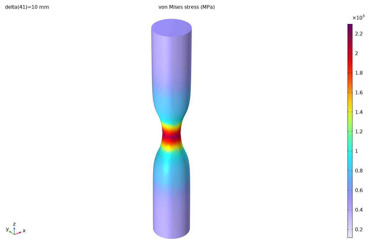
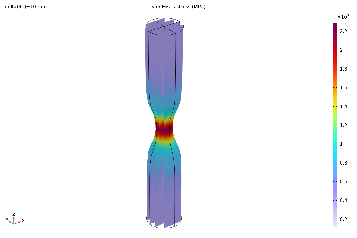
von Mises Stress Distribution
At maximum displacement (10 mm), the stress distribution clearly shows the necked region:
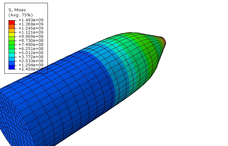
Both simulations capture the characteristic hourglass shape of the necked bar. The stress concentration at the neck center is clearly visible.
Equivalent Plastic Strain
The plastic strain distribution reveals the extent of necking:
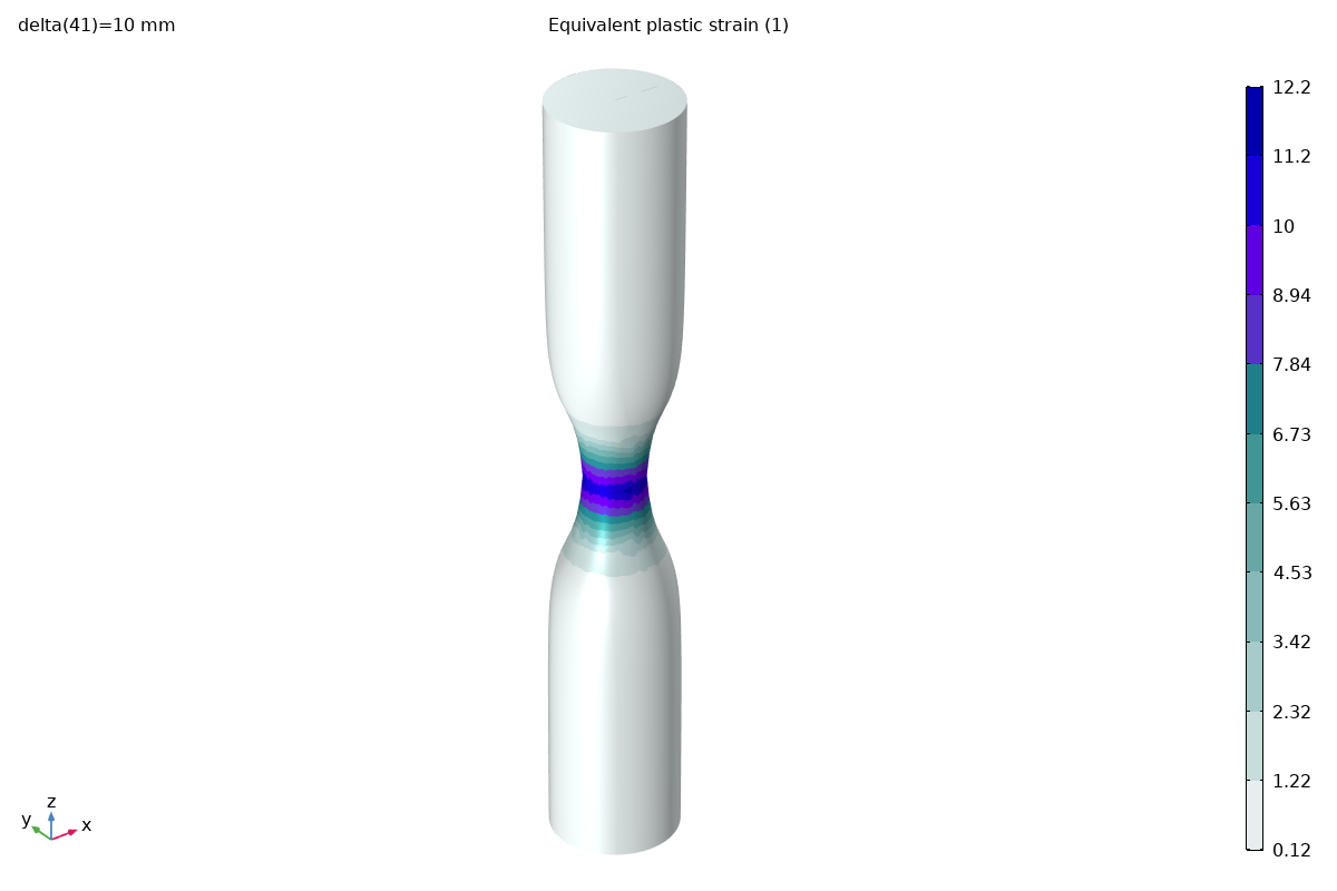
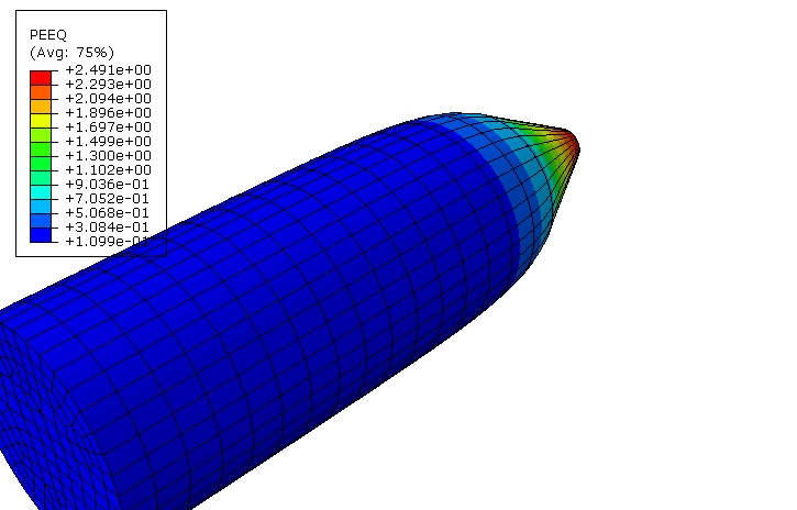
The plastic strain is highly concentrated at the neck, with values exceeding 1.0 (100% strain) near the center. This demonstrates why the large-strain formulation is essential.
Force-Displacement Response
The reaction force at the top face traces the characteristic curve of a necking bar:
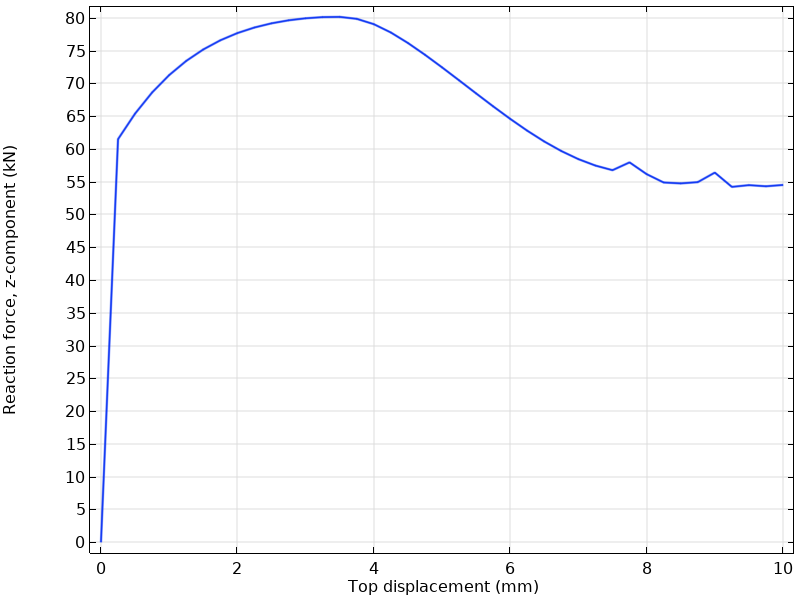
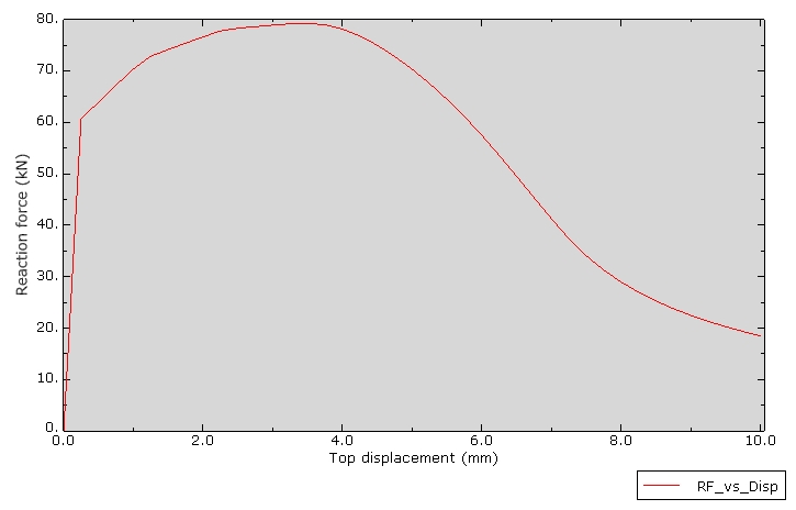
Key observations:
- Initial elastic response: Linear region up to yield (~450 MPa)
- Hardening phase: Force increases as the material strain hardens
- Peak force: Maximum load-carrying capacity (~60-65 kN)
- Post-peak softening: Force drops as necking progresses and cross-section reduces
The peak force location corresponds to the Considère criterion being satisfied—the onset of geometric instability.
Neck Radius Evolution
Tracking the radial position of a point on the neck surface shows the progressive constriction:
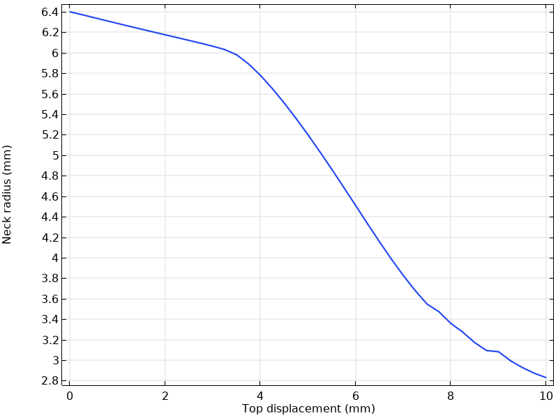
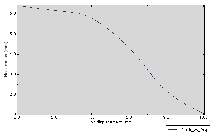
The neck radius decreases from the initial 6.4 mm to approximately 4-5 mm at maximum displacement, representing a significant (>30%) reduction in cross-sectional area.
Cross-Section View (COMSOL)
COMSOL’s slice plot provides insight into the internal stress distribution:
This view reveals that the highest stresses occur at the core of the neck due to the development of significant triaxial tension (the Bridgman effect), while the surface experiences a lower stress state.
Key Takeaways
Modeling Considerations
- Geometric imperfection is essential: Without it, the simulation would not converge or would show spurious modes.
- Large strain formulation required: Small-strain assumptions fail when strains exceed 100%.
- Mesh refinement at neck: Adequate resolution in the localization zone is critical for accuracy.
- Consistent element choice: Both platforms use 10-node tetrahedra to avoid volumetric locking in plasticity.
Platform Comparison
| Criterion | COMSOL | Abaqus |
|---|---|---|
| Ease of scripting | MATLAB syntax, verbose API | Python, object-oriented |
| Hardening definition | Analytic (flexible) | Tabular (explicit) |
| Parametric studies | Built-in, elegant | Requires loop or scripts |
| Post-processing | Integrated, customizable | Separate ODB + viewer |
| Solver robustness | Good with auto-damping | Excellent for large strain |
Summary
The necking of an elastoplastic bar is a classic validation benchmark that tests a code’s ability to handle:
- Large strains and rotations
- Material nonlinearity with hardening saturation
- Geometric instability and localization
Both COMSOL and Abaqus successfully capture the necking phenomenon, producing qualitatively identical results. The choice between platforms often comes down to:
- Workflow preference: MATLAB vs Python scripting
- Ecosystem: Multiphysics needs (COMSOL) vs dedicated structural capabilities (Abaqus)
- Industry requirements: Certification and regulatory considerations
References
- de Souza Neto, E. A., Perić, D., & Owen, D. R. J. (2008). Computational Methods for Plasticity: Theory and Applications. Wiley.
- COMSOL Multiphysics Application Gallery: “Necking of an Elastoplastic Metal Bar”
- Simo, J. C., & Hughes, T. J. R. (1998). Computational Inelasticity. Springer.
- Abaqus Analysis User’s Guide: “Plasticity for Metals”
- Bridgman, P. W. (1952). Studies in Large Plastic Flow and Fracture. McGraw-Hill.